First consider the effect that limiting demand to 10000 connections per year will have on the model. Sketch what effect you think this will have on Service Demand, Installed and Incremental Units, Capital Outlay, Capital Charge and Running Costs.
-
Load the POTS model into the Editor, if it is not already loaded. Use the Save As command from the File menu and save the model as POTS_1.
-
Open the Market Segment Details dialog and then the Size dialog to show the Interpolated Series for Households. Select the Years 2002 and 2020 in turn, and delete them. Note that the Values for each year are deleted with them. Remember that the Value will now remain at 10000 up to the end of the model run period.
- Close the dialog and select the Save and Run command from the File menu (or press <F5>).
-
Look at the same graphs that you looked at previously. Do the outputs match your predictions?
If you have results for both models open, you can draw the results from both models on one graph. You might also choose the Difference option to display the differences between the two models explicitly.
Note: in order to keep the results from the first model open, do not close the current workspace before proceeding when prompted to do so. Alternatively, the results can be re-opened in the new workspace.
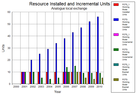
Comparison of POTS and POTS_1
Note: With shorter time periods included in the run period, it is possible to define changes in demand by quarter or month, thus providing more control over the precise timing of new equipment installation – see 10.3.30 Shorter time periods.