A very common opex element of network equipment models is power consumption. Typically a multiplier transformation is used to determine the (instantaneous) power consumption per unit of a given resource (such as a switch or router or whatever). In earlier versions of STEM, the only viable approach was to define an associated
Power
resource with (persistent) capacity of (say) 1kW. Its unit cost would have to be defined as the cost of providing 1kW non-stop for a year (which would then be billed in proportion to the length of each period and the utilisation in that period).
Given the introduction of the consumable resource in STEM 7.3, it is obviously preferable to have an
Energy
resource with (consumable) capacity of (say) 1kWh. Its unit cost would then be defined directly as the cost per kWh. However, according to the strict separation suggested so far, you would have to first use a
Time Factor
transformation to calculate the (aggregate) required energy each period in kWh before mapping this onto the actual
Energy
resource.
It is intuitive to think of the ‘h’ in kWh is an attribute of the capacity, rather than the demand, and to this end an optional
Capacity Period
can be defined for a consumable resource which tells STEM ‘how long its capacity lasts’. In other words, its consumable capacity corresponds to some kind of instantaneous measure (power) sustained for a specific period of time (an hour). This time-dependent behaviour is enabled by setting an associated
Time Factor
input to Yes as an explicit opt-in.
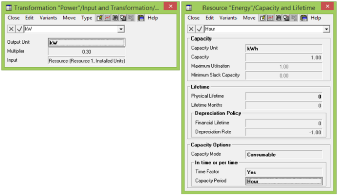
Figure 1: Mapping an instantaneous Power
demand to an in-time consumable Energy resource
The instantaneous demand must be scaled by the length of current period as a multiple of the length of the
Capacity Period
in order to infer the effective aggregate demand for the consumable resource in kWh; e.g., kW × (hours per current period). This aggregate demand is then divided into the nominal capacity in kWh in order to calculate the number of billing units consumed in the current period. The calculations are exactly as if the
Time Factor
transformation suggested above were incorporated into the resource.
The Energy
resource is still consumable in the sense that its capacity is used up and is aggregated across periods when consolidated in the results, but we shall refer to it as an
in-time consumable resource
to reflect the implicit time factor which allows it to be driven by an instantaneous demand.
Matching (aggregate) hours required to (persistent) engineer capacity per week
Just like the Time Factor
transformation, there is an inverse case in which a Capacity Period
can be used to allow a persistent resource to be driven by an aggregate demand. Recall the conversion from aggregate to instantaneous which we did to compare contracted aggregate maintenance costs with instantaneous capacity of salaried engineers.
If you have an aggregate demand of hours required for maintenance tasks, you could map this directly to a persistent
Engineer
resource with a capacity of tasks per month or more generally with a capacity of hours per week (or whatever). The subtlety here is that it is not the aggregate tasks or hours which are factored, but the ‘per week’ or ‘per month’ part. (Note it is per week as opposed to for an hour as per the energy example.)

Figure 2: Mapping an aggregate Tasks
demand to a per-time persistent Engineer resource
The aggregate demand must be divided by the length of the current period as a multiple of the length of the
Capacity Period
in order to infer the effective instantaneous demand for the persistent resource in tasks or hours per week; e.g., tasks or hours / (weeks per current period). Then this instantaneous demand is divided into the nominal capacity in tasks or hours per week in order to calculate the number of engineers required in the current period. Again the calculations are exactly as if an inverse
Time Factor
transformation (Output Mode =
Instantaneous Rate) were built into the resource.
The Engineer
resource is still persistent in the sense that its instantaneous capacity of tasks or hours per week is ongoing, rather than being used up. When consolidated in the results, we take the last period value for
Used Capacity. We shall refer to it as a per-time persistent resource
to reflect the implicit time factor which allows it to be driven by an aggregate demand.
These classifications and dynamics are compared more succinctly in the table below:
| Persistent resource | Consumable resource |
| Instantaneous demand |
A persistent resource provides ongoing capacity to support instantaneous demand
(Time Factor = No, the default)
|
An in-time consumable resource provides capacity for a period of time which is used by instantaneous demand for the duration of the current period (Capacity Period
= Hour; e.g., kWh)
|
| Aggregate demand |
A per-time persistent resource provides ongoing capacity to support aggregate demand per given period of time (Capacity Period = Week; e.g., tasks or hours per week)
|
A consumable resource provides capacity which is used up by aggregate demand in the current period
(Time Factor = No, the default)
|
Figure 3: Comparing resource capacity modes and periods for instantaneous and aggregate demands