Net present value (NPV) is the discounted cumulative cashflow generated by a business over the lifetime of the investment, and measures the value of the business based on the money it will generate in the future.
The net present value of the investment up to year n, NPVn, is calculated as:
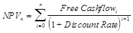
The Free Cashflow result used is the Cashflow before Financing with Net Interest Expense and Change in Investments added back, so that the net present value result does not depend on the financial structure (gearing) of the business.
The Discount Rate, r, is a value defined in the Editor (global Financial Data dialog), and is a measure of risk and uncertainty, i.e., $1 today is worth more than $1 tomorrow.
If the Discount Rate is changed in the Editor and the model is run, any NPV graphs in the Results program are updated to reflect the new value.
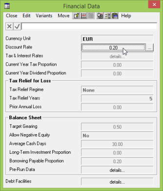
Figure 1: Changing the Discount Rate input in the Editor
The following figure illustrates how a typical Net Present Value graph is affected by choosing different values for the Discount Rate.
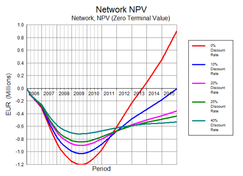
Figure 2: Net Present Value for various discount rates
Note: All of the valuation results described in this section are included as an output table,
npv.xls
, in the standard results configuration,
default.cnf.
Note: The definition for NPV supplied in the default configuration,
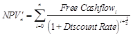
default.cnf, applies the Discount Rate as given to the first year cashflow. However, some people prefer to discount the first year by only half the Discount Rate, to allow for the fact that the cashflow comes in gradually over the year, as shown for NPV’ below.
Note: Another more sophisticated refinement would make an allowance for the extra tax which would have been paid if there had been no interest expense. This is implemented by multiplying the Net Interest Expense which is added back into the Free Cashflow result by one minus the Tax Rate.
Note: If you wish to experiment with these modifications, select Define Results from the Config menu in the Results program – see 5.17 Defining results.
Terminal value
The NPV result described above makes no allowance for the so-called terminal value of a network, which is a projection of the future worth of the network beyond the model run period. Two results are calculated, which add in two alternative estimates of the terminal value:
- NPV (EBITDA Multiplier) includes a terminal value based on a multiple of the final year EBITDA (earnings before interest, tax, depreciation and amortisation)
- NPV (Perpetuity Rate) includes a terminal value based on growth to perpetuity.
For clarity, the basic result is called NPV (Zero Terminal Value).
Both the EBITDA Multiplier and Perpetuity Rate, which govern these terminal-value calculations, are constants defined in the results configuration; you can select Constants from the Edit menu in the Results program to change the value of these constants when the corresponding Network NPV graphs are displayed. The graphs are updated automatically to reflect the new values.
Note: Each of these results is calculated as a time series which, for a given year, represents the net present value of the cashflows up to and including that year. It is useful to see how much variation there is in the results which include a terminal value in the last few years of a model, as the projected terminal values will probably be unreliable if there is significant fluctuation.
The perpetuity calculation assumes that the Free Cashflow result will grow at the Perpetuity Rate in the years beyond the run period. Thus the Perpetuity Rate is normally set close to the long-term growth rate of the economy. Assuming that the Perpetuity Rate is less than the Discount Rate, the discounted cashflows will form a bounded geometric progression, which can be easily evaluated:
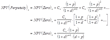
where
Cn
= Free Cashflow result in year n
p =
Perpetuity Rate constant
d = Discount Rate constant.
Break-Even Point (ZTV)
The derived result Break-Even Point (ZTV) measures the elapsed time required for the NPV to break even – that is, when the NPV crosses zero on the y axis. More precisely, it returns the elapsed time from the beginning of Y1 to the end of the most recent period when NPV (Zero Terminal Value) goes non-negative if it has previously been negative.
This result is most useful in generating snapshot tables, as illustrated below.
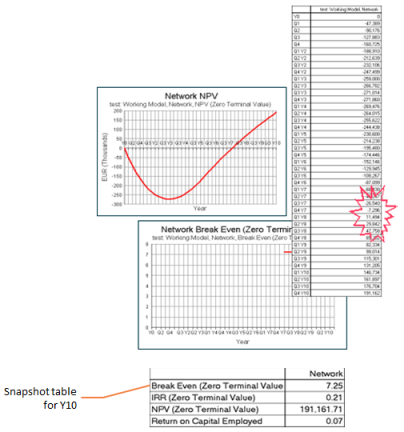
Figure 3: The Break Even result in a snapshot table
The Break-Even Point (ZTV) result is calculated from NPV (Zero Terminal Value) using the breakEven() function which returns the elapsed time to the end of the most recent period when its argument goes non-negative if it has previously been negative.
Internal rate of return
Closely related to net present value is the Internal Rate of Return (IRR) which, for a given year,
n, is the discount rate (if any) which gives NPVn = 0.
The IRR result makes no allowance for the so-called terminal value of a network; and two further results calculate the discount rates (if any) which, for a given year, give a zero valuation overall, including two different terminal values:
- IRR (EBITDA Multiplier) gives a zero valuation which includes a terminal value based on a multiple of the final year EBITDA (earnings before interest, tax, depreciation and amortisation)
- IRR (Perpetuity Rate) gives a zero valuation which includes a terminal value based on growth to perpetuity.
For clarity, the basic result is called IRR (Zero Terminal Value).
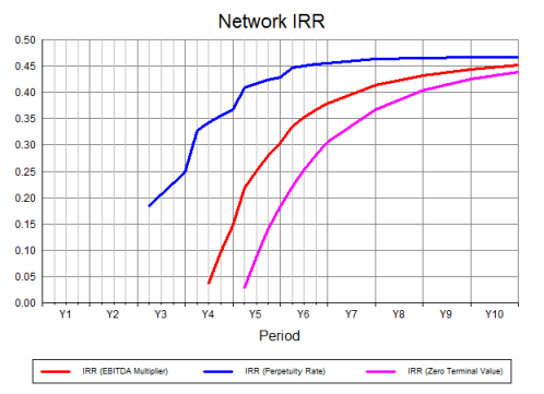
Figure 4: IRR with Terminal Values
Given the complexity of the cumulative NPV calculation, there is no closed form for IRR, and an iterative algorithm is used instead, which is effected once the central iteration for the financial model is complete – see 10.3.12 Financial model and network funding.
For a given year n, make two initial guesses for the discount rate, d: dMin
= 0 and dMax = 10. These are deliberately extreme. If NPV (dMin) and
NPV
(dMax) have the same sign, there is no solution, and so set IRRn
= #N/A. Otherwise do a ‘binary chop’ to find the intermediate value, dMid, for which NPV(dMid) = 0.
This involves setting dMid = (dMin + dMax) / 2, and then looking at the sign of NPV(dMid
). If it is the same as the sign of NPV(dMin), set dMin =
dMid, otherwise set
dMax
= dMid, and then repeat. The interval [dMin,dMax] containing the desired solution shrinks exponentially and iteration halts once this interval reduces to the order of the convergence limit specified in the Calculation Options dialog in the Results program – see 4.12.4 Using iteration to resolve circular references.
The implementation in the standard results configuration,
default.cnf, has some technical complications which are of interest only to the very technical!
The algorithm is encoded as a series of circular derived results whose definitions include some strange terms which guarantee that the iteration will process the equations in the right order, regardless of which result you ask to calculate first. For example,
dMid
is defined as:
dMid = 0 · iD + (dMin
+ dMax) / 2
where
iD = a trip variable used to seed dMin and dMax.
The ‘0 · iD
’ term has no impact on the calculation other than to force iD to be calculated before
dMid. Each of the related circular results has at least one such term.
The standard NPV (Zero Terminal Value) result is calculated from the constant Discount Rate result, and is defined cumulatively using the prev() function. However, the iteration described above has to be performed for each year separately, to calculate
IRRn. We therefore cannot use the previous year’s value for NPV(dMid) as the basis for the cumulation, as we expect dMid to vary with time.
Instead we have had to define two new primitive functions, csum(x), which gives the cumulative sum of an expression, x; and yearC(y), which returns the current year value of a term, y, within an expression, x, in the scope of a csum. These are used to define NPV(dMid) as:
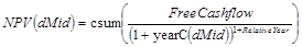
so that for the result in year n, we get the cumulative sum of Free Cashflow discounted by the value of dMid in year n, rather than the different values of dMid in the years up to and including year n.
Note: The iterative algorithm for IRR employs ten or so intermediate results. These have been hidden in the
default.cnf
supplied with STEM, as have the corresponding intermediate results for the new IRR results. If you want to unhide these, or hide any other results, select Select Results… from the Config menu in the Results program – see 5.20.3 Limiting the results available in a configuration.