STEM lets you build models with minimal input, through the use of parameterised time series, e.g., Interpolated Series, which can prescribe the full evolution of an input over time without specifying data for every year. A fundamental design criterion for the shorter time period system was that it should be as easy to use as the annual system; specifically, that you should not have to enter sub-annual data unless you want to.
Steps in conventional input data
As you have already seen, the introduction of shorter time periods immediately leads to more detail in results if the existing time-series parameterisations are evaluated without constraint. In the case above, this is because STEM uses interpolated values for the penetration in the periods within 2001. There may be occasions when it will be convenient or even essential to suppress this detail:
-
to simplify the dynamics of a model
-
for backwards compatibility
-
for greater realism, e.g., when modelling annual tariff changes.
Each individual time-series parameterisation has a new Step input which allows you to constrain the dynamics of any time-series input to yield a constant value throughout quarterly, annual or even indefinite periods. If you set Step =
Year
for the penetration input above, you will see that STEM calculates a constant penetration of 20% throughout Jan, Feb and Mar, Q2, Q3 and Q4 2001.
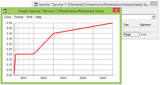
Figure 1: Interpolated series stepping in Years
Implicit and explicit alignment
The conventional STEM interpretation of annual demand data is that they represent end-of-period values. In the simple model above, we prescribed that penetration would reach 40% in 2002, implicitly taken as by the end of 2002. If we now set the run period input Years in Quarters =
2
and set the Step input back to Day, you can see that STEM infers a penetration of 40% for [the end of] Q4 2002, with lower values in Q1, Q2 and Q3 2002.
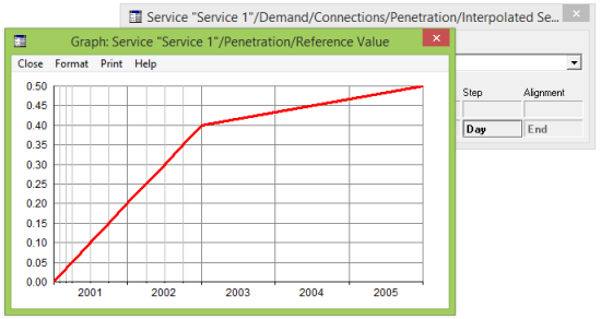
Figure 2: Implicit End Alignment
Each individual time-series parameterisation has a new Alignment input, and you can see that the default Alignment for penetration is
End. If you actually have beginning-of-period data, then you can set Alignment =
Beginning
to force STEM to associate given values with the beginning of the corresponding periods, and infer a penetration of 40% by the beginning of Q1 2002, with higher values in Q2–Q4.
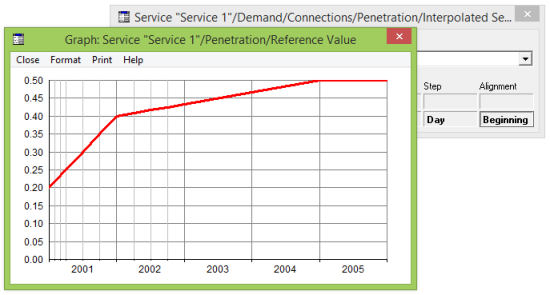
Figure 3: Explicit Beginning Alignment
However, it is very important to understand that the model engine will continue to use end-of-period values for demand. Indeed, it must use a consistent set of assumptions in order to validate the calculations it makes. This is reflected in the graph, where you can see that STEM infers a penetration of 40% for [the end of] Q4
2001, which of course coincides with beginning of 2002 as specified.
Fortunately, these considerations are only relevant if you need to specify inputs with unconventional Alignment. In fact most inputs have implicit
End
Alignment, the only exceptions being tariff and cost trend inputs.
Adding quarterly data
Suppose now that we want to be more specific about the initial penetration, say only 4% at the end of the second quarter, compared with the previously interpolated value of 10%:
-
Select the first empty cell in the Period row of the Interpolated Series dialog, to the right of the years
2000, 2002 and 2005, which you have already entered.
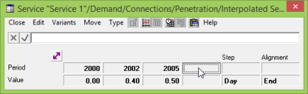
- Enter a new period literally as Q2. As soon as you press <Enter>, the data are sorted so that
Q2
appears between 2000 and 2002.
- Enter the corresponding value as 0.04.
The graph changes to reflect the new value for Q2 2001, and the correspondingly lower interpolated values for Jan, Feb and Mar 2001. Because this input has
End
Alignment, the value of 2% for Mar 2001 is exactly half the value of 4% for the end of Q2 2001, i.e., Jun 2001.
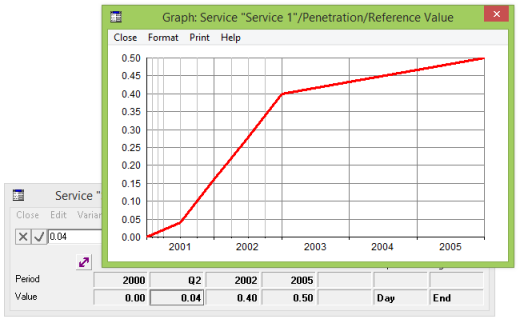
Figure 4: Interpolated Quarterly Data
Specifying relative years
STEM interpreted the Q2, entered above, as the second quarter from the Model Start Date. In this case, the Model Start Date, entered as
2001, is equivalent to 1 Jan2001; relative to which, Q1
means Jan–Mar 2001, Q2 means Apr–Jun 2001, and so on.
On a similar basis, you can enter Yn to represent the nth year following the Model Start Date for any integer n
< 1000, which in this case means that Y1
is identified with 2001. Year zero, the optional base year, is the year before the Model Start Date. The unqualified input Q2
is equivalent to Q2 Y1.
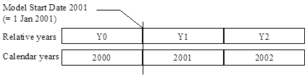
Figure 5: Relative Years and the Model Start Date
Note: This represents a change in the semantics of relative year inputs from STEM 5.4, where year zero was identified with the Model Start Year.
If you enter a non-negative integer < 100 for a period input without a leading
Y, then by default STEM infers an appropriate century, e.g., 1
is taken as the absolute calendar year 2001, whilst
99
is taken as 1999. This is conventional behaviour for entering dates, and governed by a new menu item, Infer Century, on the Options menu in the Editor. If you would prefer an unqualified
1
to be taken as the relative year Y1, as in STEM 5.4, then simply de-select the Infer Century option.
Note: Unqualified negative integers are always interpreted as relative years.
Adding monthly data
With the default End Alignment for penetration, the input
Q2
is equivalent to Jun. Now suppose we want to be even more specific about the Service take-up by the end of Apr, say at a level of 2%, compared with the interpolated value of 2.7%:
-
Re-enter the period Q2 as Jun. The values on the graph are unchanged.
-
Enter a new period as Apr with a corresponding value of
0.02. Now the graph shows different values for Jan, Feb and Mar 2001, but Apr is not shown.
-
Set the run period input Quarters in Months = 2
to reveal Apr, May and Jun.
- Select Show Graph As Table from the Format menu to examine the values.
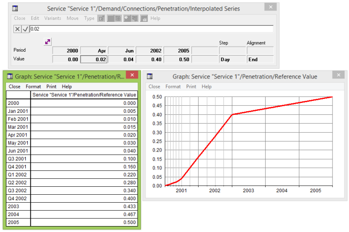
Figure 6: Interpolated Monthly Data
The penetration grows in monthly steps of 0.5% to a value of 2% at the end of Apr, and then in 1% steps to 4% at the end of Jun. Growth continues at 6% per quarter to 40% at the end of 2002, and then slows in the subsequent years as before.
Capturing changes on specific dates
The end of Jun can also be specified explicitly as [the end of]
30 Jun, and if you wish, you can enter any arbitrary fully-qualified date within the idealised calendar. As mentioned above, the new
Indefinite
Step option provides the facility to specify an irregular series of step changes, which might be especially useful for entering tariff changes:
- Select Tariffs from the Service icon menu. The Tariffs dialog is displayed.
- Click the Rental Tariff button.
-
Right click and select Interpolated Series on the Change Type context menu.
-
Enter the dates 1 Jan 2001 and
17 Mar 2002, with respective values
25
and 22.
-
Click on the
 button to draw a graph of the Rental Tariff. Intermediate values are interpolated by default.
-
Set Step = Indefinite
in the Interpolated Series dialog. From Jan 2001 up to and including Q1 2002, the tariff is now constant at
25, only stepping down to
22
in Q2 2002, the first period beginning on or after 17 Mar 2002.
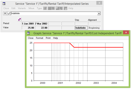
Figure 7: Specifying an Irregular Series of Step Changes
In this example, STEM calculates revenue as if the tariff were constant throughout Q1 2002. In a future release, we might aim to partition the specified run periods at any intermediate dates, but this is beyond the scope of the current system.
Note: If you set Step = Indefinite
for an input with Alignment = End, then the input will retain the value specified for a given date for periods up to and including the
last
period ending on or before that date.