The introduction of shorter time periods immediately leads to more detail in results if conventional annual time-series parameterisations are evaluated without constraint, perhaps for example because a range of interpolated values are used for successive quarters of a year. There may be occasions when it will be convenient or even essential to suppress this detail:
-
to simplify the dynamics of a model
-
for backwards compatibility
-
for greater realism, e.g., when modelling annual tariff changes.
Each individual time-series parameterisation has a new Step input which allows you to constrain the dynamics of any time-series input to yield a constant value for quarterly, annual or even indefinite periods. Although the basic semantics of this input are the same in all parameterisations, additional points are noted for the more complex types.
Stepped Exponential Growth
By default, the input Step = Day for any time series, which means that the time-series parameters are evaluated without constraint. So for an Exponential Growth with, e.g., Base =
1, Multiplier = 1.05, Base Period = Y1
and Alignment = End, a value of 1.0 will be calculated for the end of Y1 and appropriate, slightly lower, values for Q1, Q2 and Q3 if the run period input Years in Quarters =
1.
If you set Step = Year, this directs the calculation to yield a constant value for each year. Specifically, the calculation returns the Base value for a period of a year to the end of Y1, and then 1.05 throughout Y2, and so on, so that the value is constant from Q1 to Q4 – see Figure 1 below. (These annual steps are most evident if you set Years in Quarters = 5.)
If you set Step = Quarter, different values will be used for Q1 to Q4; but if you set the run period input Quarters in Months =
1, you will see that the values for Jan and Feb are constrained to match the Mar value so that the input is constant throughout the quarter.
Note: If you set Step = Month, the results will appear unconstrained because the current shorter time period interface only provides for quarters and months in the model run. Further detail may be allowed in a future release.
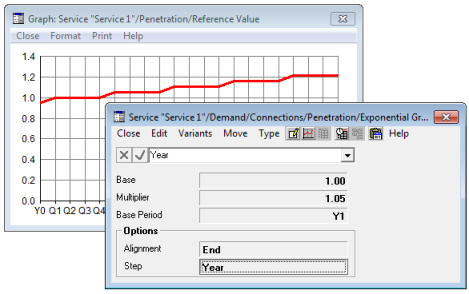
Figure 1: Exponential Growth stepping back in Years
Each constant step runs to the unconstrained value at the end of a period if the input has Alignment =
End, so that the nominal Base value for the end of Y1 applies to the whole of Y1. However, if the input has Alignment =
Beginning, then the constant steps run forward from the unconstrained value at the beginning
of a period. With the same example, you will see a value of 1.0 for Jan (the beginning of Y1) and the same constant value for Feb and Mar, before increasing in Q2.
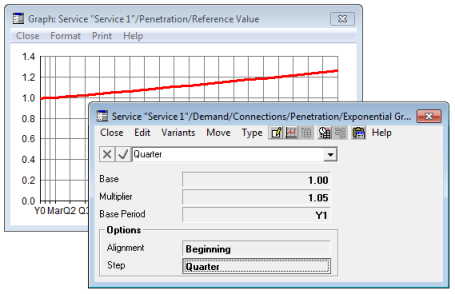
Figure 2: Exponential Growth stepping forwards in Quarters
Stepped S-Curve
If you define Step = Year or Quarter
for an S-Curve then, as for the Exponential Growth, you will see the calculated values run along in constant steps between the calibration periods, namely the Base Period, Period A and Period B. The only complication arises if the number of ‘steps’ between a pair of these periods is not a whole number. For example, if an S-Curve is defined with Saturation =
1.0, values 0.1 in Y1 and 0.5 in
Q2
Y3, Alignment = End and Step =
Year, then there is only a year and a half from the calibration point for Value A to that for Value B.
This conflict is resolved by the argument that it would be grossly counter-intuitive for the input not to assume Value A in Period A and Value B in Period B, and that therefore these calibration points must override the stepping. To be precise, with Alignment =
End, annual steps run back from the end of Period B until the end of Period A, and annual steps run back from the end of Period A; but it may be necessary to truncate the step from Period B which runs back to Period A, and similarly the step from Period A which runs back to the Base Period.
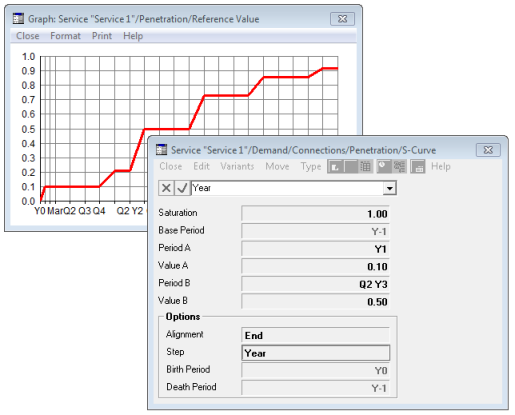
Figure 3: S-Curve stepping back in Years
So in this example, the constant
value 0.5 pertains
for a year
from Q2 Y3
back to Q3
Y2, but then
the next step
back from the
end of Q2
Y2 is truncated
to half a
year so that
the calibration value
of 0.1 can
pertain for a
year back from
the end of
Y1.
If, on the other hand, you set Alignment = Beginning, then you will see annual steps for Y1 and Y2 and then a truncated step for Q1Y3, prior to annual steps from the beginning of Q3 Y2.
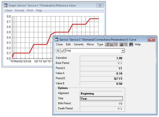
Figure 4: S-Curve stepping forward in Years
Stepped Interpolated Series
As with an S-Curve, the Step input can be used to generate a series of stepped values between the given calibration data for an Interpolated Series, and there is a similar complication if the given calibration periods are not a whole number of ‘steps’ apart. Again, this is resolved in favour of the calibration data: one intermediate step may be truncated if it runs into the next calibration period.
There is an additional choice, Step = Indefinite, which causes an input to assume a constant value from one calibration period to the next, allowing you to specify an irregular series of step changes, which may be especially useful for entering tariff changes on specific dates. For example, if you first set run period input Years in Quarters =
2, and then define Service Rental Tariff as an Interpolated Series with values
25
on 1 Jan Y1 and 24 on
17 Mar Y2, intermediate values are interpolated by default; but if you set Step =
Indefinite, the tariff is now constant at 25, only stepping down to 24 in Q2 Y2, the first period beginning on or after 17 Mar Y2.
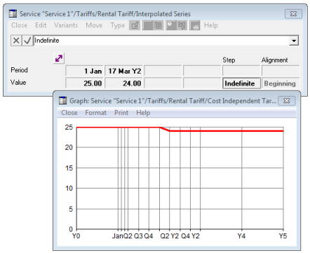
Figure 5: Interpolated Series stepping indefinitely
Note: Although the Indefinite
choice is available for all parameterisations, it is only intended for Interpolated Series; and of course the term ‘Interpolated Series’ is a bit of a misnomer when Step =
Indefinite. However, it seemed more intuitive to provide this functionality as an Interpolated Series that doesn’t actually interpolate, rather than as a separate item on the Type menu.