The existing Time Lag transformation was added to STEM in the days when models could only run in years and has been used most commonly to drive ‘difference relations’ or to avoid circularities. When shorter time periods were introduced, it was clear the Lag input (years) should be respected, and so the output always looks back the n years and skips any intermediate months or quarters. However, this offers no way to refer to an immediately preceding sub-annual period which could be used safely for a difference relation.
The Previous transformation allows modellers access to values from the preceding time period, no matter what time periods are used. The optional Costs input is used to avoid circular cost-allocation, just as it is for the Time Lag transformation. There is also an optional Multiplier time-series input that can be used to scale the output, and an Output Unit input that can be used to specify a label for the output.
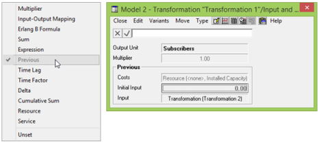
Figure 1: Transformation Type menu and Previous transformation dialog
An example of the output of the Previous transformation is shown in the table below. The input (the top row) is a constant-growth time series, increasing at 1000 units per year (or 250 units per quarter). The output (the bottom row) is the same as the top row, except delayed by one period.
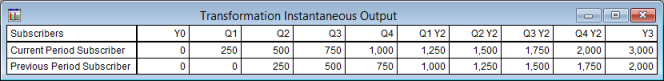
Figure 2: Example output of the Previous transformation
The value of the output in Y0 is specified by the Initial Input value (zero in this example).
By default, the present costs of any dependent Resources (secondary costs) are passed back through to the input of the transformation (see 10.3.4.1 Allocating costs through Transformations). However, if the transformation is involved in any kind of circular difference equation, where the reference to a previous value resolves the apparent circularity, then the optional Costs input should be used to specify a separate element to which STEM can allocate the secondary costs.