Each element in the model is characterised by the associated input data, which is presented in a set of data dialogs. In order to access one of these dialogs:
-
Double-click or right-click on the icon representing the resource labelled Eight channel base station. A pop-up menu appears.
-
Select Capacity and Lifetime from the categories of data listed in the top section of the menu. The Capacity and Lifetime dialog opens.
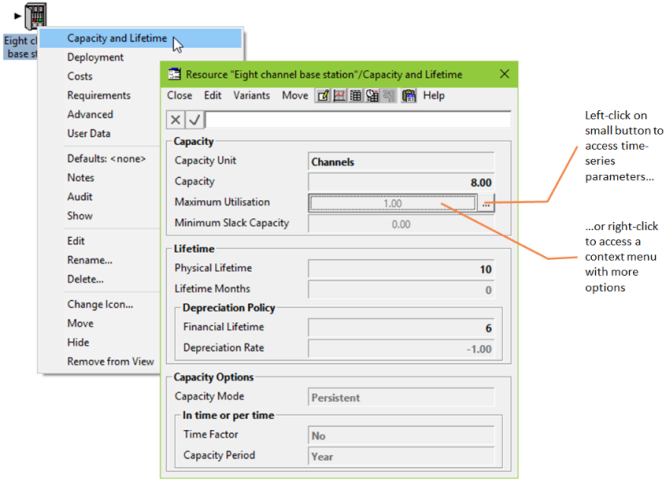
Accessing Capacity and Lifetime data for a resource
The Capacity Unit, Capacity, Physical Lifetime and Depreciation Policy are displayed in the cells in the dialog, and can be modified using the formula bar. The Maximum Utilisation and Minimum Slack Capacity fields are time-series inputs, a summary of which is displayed in the cells. When a time-series field is selected, a small button appears to the right which you can left-click on to access the time-series parameters. Alternatively, you can right-click to access a local context menu with more options for the selected field. Select Close from the dialog menu bar to close the dialog.
Dialogs for other elements of the model or other categories of data can be opened using the same procedure. Notice also that if you place your mouse cursor over an icon for more than a few seconds, a concise summary of the data set within that element is displayed. Before proceeding further, we suggest you spend some time browsing through the model data. The following items provide a brief introduction to a range of factors that a STEM model can take into account.
 Market Segments
Market segments represent the different groups of customers that may use the services within the model. Demand for a service can be represented by the level of penetration of the service into the size of a market segment.
From the icon menus for Residential Households and Small and Medium Businesses, select Details to view the Size input and look at:
-
How the number of potential subscribers is influenced by the Base station site plan element. In the formula bar, we use an internal reference to link the size of the market segments to the size of the coverage area.
-
How the number of residential households and businesses in the coverage area is increasing with time. In particular, click on the graph button
 to see the growth in both line types.
 Services
Services represent the services offered by operators to their customers, such as ISDN, voice mail, X.25 or international calls. The demand for each service is specified in terms of connections, the annual traffic and the busy hour traffic. Tariffs are specified for each service, which STEM uses to calculate revenues. A service can have a Connection, Rental and a Usage Tariff. A Churn Tariff can also be specified if required.
From the icon menu for Residential PSTN, select Demand and look at:
-
Penetration: the proportion of homes passed that subscribe to the wireless service, defined as an S-curve. Click on the graph button and select Auto Graph
to see the shape of this curve.
-
Traffic per Connection: represents both the incoming and outgoing annual traffic in Call Minutes per connection per year, defined as an interpolated series. The value in the first year is based on eight minutes per day for both incoming and outgoing calls for 365 days per year.
 Resources
Resources represent particular types of equipment (e.g., a telephone handset, an ATM switch or a vehicle) or other sources of cost in the network to be modelled.
A resource is described in terms of its physical characteristics and costs. These include its Physical Lifetime, Capacity, and the various costs of ownership or use (e.g., Capital Cost and Maintenance Cost).
From the icon menu for Microwave System, select Costs and look at:
-
How the annual Maintenance Cost is defined as a percentage of the initial Capital Cost.
-
The other types of resource costs that you can define within STEM.
 Transformations
Transformations are used to represent special relationships between calculated quantities in the model. They can, for example, be used to relate the required capacity of one resource to the installed capacity of another, potentially in a non-linear way. They can also be used to relate the use of a service to the installed capacity of a resource. Another important type of transformation is the Erlang B Formula, which is used to convert the busy hour traffic demand of a service into the resource capacity which needs to be installed.
From the icon menu for Backhaul Transmission, select Resources Required, and then select the Transmission Facilities function. Look at:
-
The split between the two types of backhaul transmission system used in the network, i.e., Leased Line and a proprietary Microwave System.
-
How the transition from Leased Line to Microwave System is performed between year 0 and year 5.