2.1.6 Exploring the likely range for resource deployment

You can change the settings in STEM to make the resource deployment more realistic:

1. Return to the STEM Editor.
2. Right-click on Resource 1 and select Deployment to access the Deployment dialog (or right-click on the blue line connecting Location 1 and Resource 1 and select Details).

In the Distribution field of the Deployment dialog you can choose from one of five assumptions about how demand is spread across sites, which affects how STEM calculates the number of resources required to meet demand. For a description of each option, go to  Resource / Deployment.

Note: pressing <F1> at any time when using STEM will take you to the relevant Help topic in our online Help site.

Homogeneous distribution

In this example, we will explore Homogeneous distribution, whereby demand is distributed evenly across the sites, and at least one unit of resource is installed at each site. When all units are fully utilised, another unit is installed at each site.

1. Select the Distribution field. Click the drop-down button on the formula bar and select Homogeneous.

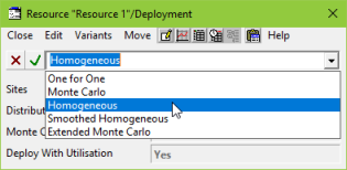
Figure 1: Changing the Distribution in the resource Deployment dialog

2. Re-run the model (by pressing <F5>).
3. Look at the Capacities results again: two resources are installed at each site once the number of customers exceeds 500.
4. Confirm this by looking at the Installed and Incremental Units graph: in Y4 an additional 10 units of resource are installed, making 20 in total.

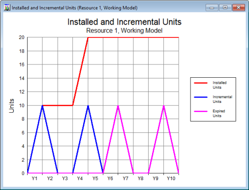
Figure 2: Installation of additional resource units with Homogeneous distribution

However, it is unlikely that each site will exceed the 50 threshold at the same time in practice, so we will now consider another type of distribution.

Monte Carlo and Extended Monte Carlo distributions

Consider a worst case scenario, in which there is one customer at each of sites 1–9, and all the other customers are located at site 10. In this instance, you would need one unit of resource at each of sites 1–9, with effectively a spare resource unit at each of these sites, and after every 50 additional customers, another unit of resource would need to be installed at site 10.

Suppose instead that you could have approximately half a unit of slack capacity at each site (25 customers slack capacity per site), making an overhead of 5 units. Statistical evidence suggests that half a unit slack capacity at each site is a reasonable overhead, and it is certainly more credible than the One for one distribution or Homogeneous distribution, or the worst case described above.

The Monte Carlo distribution will install additional site-dependent slack capacity, in addition to the minimum necessary to meet demand. The extra slack capacity installed corresponds to an average of half a unit at each site. Let’s try it!

1. Return to the STEM Editor.
2. Select the Distribution field. Click the drop-down button on the formula bar and select Monte Carlo.
3. Run the model (by pressing <F5>).
4. Look at the Capacities graph in the results program.

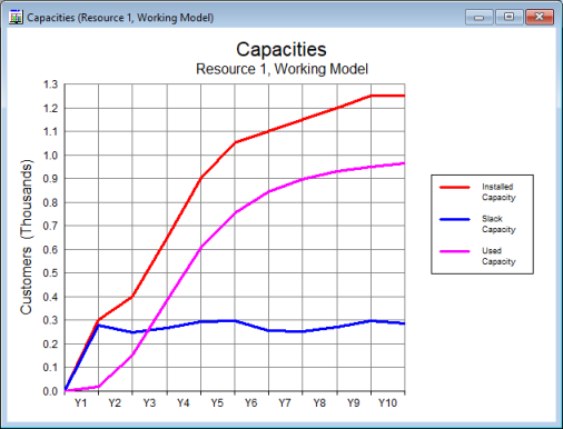
Figure 1: Effect of the Monte Carlo distribution on the resource Capacities graph

You can see that the Installed Capacity no longer increases to 1000 in Y4, but instead increases gradually. The Installed Capacity is consistently about 250–300 customers higher than the Used Capacity, which equates to roughly half a unit of resource (25–30 customers) per site.

If you also look at the Utilisation Ratio graph, you will see that this too seems realistic, as the utilisation ratio increases gradually. However, only six resource units have been installed in Y1 using this distribution, so this is not realistic if we assume that there could be some customers at each of the ten sites in Y1. The Monte Carlo distribution is assuming that, as there are only 20 customers in total in Y1, some sites may have no customers at all, so do not require any resource capacity. If you want to ensure that there is resource capacity at each of the ten sites from Y1 onwards, you can use the Extended Monte Carlo distribution, which is the same as the Monte Carlo distribution, except that at least one unit is installed at each site.

5. Return to the Editor and change the Distribution input to Extended Monte Carlo.
6. Run the model.
7. Look at the Capacities graph again.

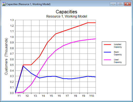
Figure 2: Effect of the Extended Monte Carlo distribution on the resource Capacities graph

Now you will see that ten resource units are installed initially (one per site; 500 customers), and that when the Used Capacity reaches 50% (250 customers) during Y3, STEM starts to install more resource units, such that there is about half a unit of slack capacity per site (250 customers in total).

The Extended Monte Carlo distribution provides a good estimate of how many units of resource to install to meet demand. In the next part of this tutorial we will examine the impact this distribution of resources has on the cost and overhead required to run the business.

© Implied Logic Limited

Comments on this help resource are welcome – please make a suggestion