Watch the video presentation and/or read the full text below
Now we are going to think more carefully about how the numbers of customers are
spread out between the various locations where equipment is installed:
-
Double-click the light-blue, location link (or select
Deployment from the icon menu for the
Access card resource). The
Deployment dialog is displayed, as shown below,
with the input
Distribution = One for One
by default. This is what determines the minimal results we have seen so far.
The only impact is that, literally, at least one unit will be installed for
each site (as soon as there is a non-zero demand). We will explore two of the
available alternatives as follows.
-
Click the Distribution field, and select
Homogeneous from the drop-down in the formula bar,
as illustrated below. This setting indicates that the customer demand should be
assumed to be split evenly between all of the sites. When the first card is full
at every site, then another must be installed at every site, and so on.
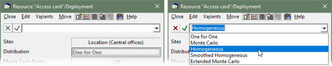
Figure 27: Changing the Distribution input in the
Deployment dialog for the
Access card resource
-
Re-run the model (still skipping warnings) and review the updated results.
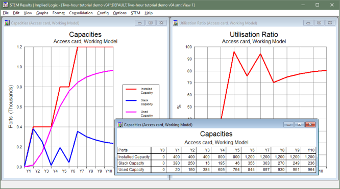
Figure 28 Capacities and
Utilisation Ratio graphs with
Distribution = Homogeneous
As soon as the demand exceeds the initial 400 ports, another 25 units are installed.
Such a distribution is unlikely in real life, but is useful as an extreme example.
In practice, it is likely that there will be ‘hot’ sites where the initial
capacity is exceeded sooner than Y3, and other ‘cooler’ sites where
this happens later. At any given site, as demand increases, the number of slack
ports will vary in the range 0–15 inclusive. Given the likely variation in
timing across sites, a fair estimate of the slack capacity required at any point
in time will amount to ‘half a unit’ per site; i.e., 200 ports. This
would have the required installation tracking some way above the pink line for
Used Capacity, cutting a more gradual path compared
to the simplistic red steps shown above.
-
Switch back to the Editor, and set the input
Distribution = Extended Monte Carlo.
-
Re-run the model (still skipping warnings) and review the impact on
the results.
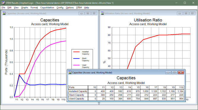
Figure 29: Capacities and
Utilisation Ratio graphs with
Distribution = Extended Monte Carlo
As you can, this setting maintains a roughly constant overhead of just over 200
slack ports beyond the number of ports actually in use at any given point in time.
Beyond the initial constraint of one unit per site, the used capacity is proportional
to the demand, whereas the slack capacity is more or less proportional to the number
of sites. This is the most prudent approach; so, if in doubt, use
Extended Monte Carlo.
(Beyond the scope of this tutorial.)
By all means experiment with the other two options for the
Distribution input:
-
Monte Carlo: as above, but without
the initial constraint of one unit per site; suitable if a ‘just-in-time’
deployment model is feasible for the first customer at each site
-
Smoothed Homogeneous: like
Homogeneous, but also without the initial constraint of one
unit per site, but only really included as an academic example for completeness.
 Things that you should have seen and understood
Deployment, Distribution, One for One, Homegeneous, Extended Monte Carlo