Watch the video presentation and/or read the full text below
Now let’s look at the results:
-
Run the model. (Still skip the warnings about the last resource which
we haven’t connected yet.) The Results program is activated.
-
Change selections for the existing Capacities
and Utilisation Ratio graphs to show the
Access chassis instead of the
Access card.
-
Draw Installed Units as a table for
Optical interface,
Access card and
Access chassis, using the option in the corner of the
Draw dialog to
Show Graph as Table.
-
Add Access chassis to the stacked
Capital Expenditure and
Operating Costs graphs.

Figure 33: Capacities and
Utilisation Ratio for the
Access chassis, plus inventory of resources
The Capacities and Utilisation
Ratio graphs may be suspicious, but it is immediately clear from the
Installed Units table (inventory) that there are
only have five chassis for 25 cards in Y1, and still only 15 chassis in Y10, whereas
we should have chassis at all 25 sites.
STEM is aware that the cards are in different places, but not that the chassis are
too. Collocation cannot be inferred from the dependency between the elements; e.g.,
some management software could be virtualised and shared in a separate data centre
location.
Therefore, we must tell STEM about the deployment of the chassis too:
-
Connect the location to the Access chassis
resource, as we did for the Access card.
-
Double-click the location link and set Distribution
= Extended Monte Carlo.
-
Re-run the model (still skipping warnings) and review the impact on
the results.

Figure 34: One Access chassis per site at the start,
and then a few more later at the busier sites
Now there is a chassis at every site from Y1, with very low utilisation at the start,
and then just a few more are added from Y5 onwards. There is an average of c. three
cards per site in Y10 (74/25), but the simulation suggests a few of the busier sites
actually need a sixth card, and thus an extra chassis. In contrast, some of the
quieter sites might only need one or two cards, but still need one, under-utilised
chassis.
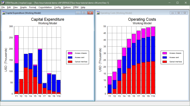
Figure 35: Stacked Capital Expenditure and
Operating Costs graphs for all the resources so far
You might wonder why the location for the cards is not based on the number of chassis.
In this example, the number of Central offices
is a given, and more than one chassis might be needed eventually at some sites,
as shown above. An extra chassis should not demand further cards; it is the cards
that need a chassis, not the other way round!
The remaining commentary explores refinements beyond the scope of this tutorial.
The number of locations is really part of the marketing plan. With more time, we
could compare the merits of a phased roll-out; perhaps launching at only five sites
(to limit the initial capex), and then adding the others gradually. This would spread
the capex, but also delay revenue, so it is not obvious which would yield the greater
return.
With more data about the distribution of potential customers, we could also model
the dimensioning of cards and chassis at individual sites, rather than estimating
the impact with the deployment feature. This can be done very efficiently and consistently
using a feature called template replication.
With such an approach, the choice of specific locations could be tailored such that
none would ever require more than one chassis. However, the number and location
of viable sites may not bear any correlation to the proximity of potential customers,
so this may not be possible in practice.
As it is, the aim for this short exercise is to keep things simple, and to estimate
the impact of geography, as you might for an initial business plan, rather than
being specific about where the chassis are. We might re-visit the ideas above in
a future sequel!
 Things that you should have seen and understood
Show Graph as Table