Exercise 28: Defining cost trends for all, and for individual, resources

For ease of understanding, the initial model has the annual Maintenance Cost as a constant over time. Now we are going to look at different ways of varying this.

Global cost trends

Suppose you are in a hurry and want to capture a general trend, perhaps that maintenance costs will increase across the board due to rising costs of labour or more environmental disposal of spare parts.

1. Locate the global Maintenance Cost Trend input for resources (Data menu/Cost Trends).
2. Right-click on the input field to access the context menu. Use the Change Type option to select Exponential Growth.
3. Set the input Multiplier = 1.05, and run the model.

Base period

4. Check the Maintenance Cost result (which should have been saved with the previous workspace). You should now see a steady increase in each period.
5. What is the value in Q1 2007? What was it without the cost trend?
6. Go back to the Editor and set the input Base period = 2007.
7. Re-run the model and see if that made any difference.

It would not be very practical if the absolute value of a global cost trend was significant, as it would imply that all resource costs were defined for the same nominal base period. Instead, the global trend is normalised for each individual resource against its own so-called calibration period.

Calibration period

8. Set the input Calibration Period = 2007 for the DSLAM chassis (icon menu/Costs) and re-run the model.

This Calibration Period input defines when constant unit costs entered above will apply when used in conjunction with separate cost trend inputs.

Local cost trends

9. Although it is convenient to use global trends, often you will need to be more specific, and there is also a separate cost trend for each individual resource (and for each of the different supported cost attributes).
10. Go to the local Maintenance Cost Trend input for the DSLAM chassis (Advanced/Cost Trends) and define an annual growth of 5% as above.
11. Re-run the model and check the results. The result should be the same for Q1 2007, but it will now be growing twice as fast.

By default, STEM combines both global and local trends for a resource. Try setting the input Use Global Trends = No to inhibit the global trend for an individual resource (icon menu/Costs).

Time-series input

Sometimes you may be given explicit time-series cost data which define the trend in actual unit costs over time. These can be entered directly into the Cost input.

12. First convert the existing formula for the maintenance cost to a constant (dialog Edit menu/Freeze).
13. Right-click the Maintenance Cost input field and Change Type to Interpolated Series.
14. Change the first period from Y0 to 2007, and then enter these values:

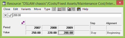
STEM will automatically insert the period for you if you enter a value in the next empty column, incrementing in years or quarters or months according to the size of the preceding period.

15. Re-run the model and look closely at the results. Check the numbers. Why does the maintenance cost decrease at first, but then increase again after 2009?

STEM provides global and local trends, as well as absolute time-series inputs, for maximum flexibility and compatibility with other data sources. Some care and consideration are required if you choose to use all of these features in parallel. The local trend and time-series inputs are mainly seen as alternative input models, but you may find a compelling reason to use both!

Of course, the same principles demonstrated for maintenance cost in this exercise apply equally to all the other cost attributes.

Service costs

You can also enter per-connection and per-incremental-connection costs for a service (Advanced/Administrative Costs), and these benefit from a similar global and local cost-trend mechanism. However, you may prefer the greater flexibility of modelling these costs with separate resources. As with all costs, these will still be attributable to the services through cost allocation, as described in more detail in 2.3.14 Service costing and profitability analysis.

Cost indexes and capital cost structure

There is also a more complicated mechanism, specifically for capital costs, which uses one or more separate cost index elements to model the production costs in more detail. However this economic technique is no longer common usage within STEM, and is beyond the scope of this training course. Please see the help resource for more details.