By default STEM takes no account of the geographical distribution of Resources. However, in reality, Resources are geographically spread as demand or the network architecture requires. STEM is able to model this real-world situation through the use of the Deployment feature. Deployments can be made on the basis of a Function or on the basis of individual Resources or both – see 10.3.18 Locations and deployment.
For the POTS model, however, with only one Function (Local Switching), the Local Exchanges are dimensioned on busy-hour traffic with no account taken of any geographical constraints.
To model the effects of Deployment, we will install the local exchanges initially at 15 sites and then add 20 more later.
- Open POTS_4 and save it as POTS_5. Double-click on the Function element icon to display the pop-up menu.
- Select Deployment.
- Enter the Time Series dialog for Sites and choose Interpolated Series from the Type menu.
- Give years 2000 and 2001 respective values of 15 and 35.
- Click the graph button to check that your graph looks as shown below.
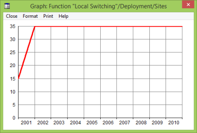
Time Series graph for Function Deployment
- Sketch the graphs you expect for Resource Installed and Incremental Units.
- Save and run the model.
Do the graphs for Resource Installed and Incremental Units match your predictions?
Look at the graph entitled Resource Capacities for the Analogue Exchange; what is this showing?