Watch the video presentation and/or read the full text below
The first thing we need to do is create a service element:
- Click the Service button
 on the toolbar, and then click again to place the ghosted icon at a suitable position
in the view. The service element is created.
on the toolbar, and then click again to place the ghosted icon at a suitable position
in the view. The service element is created.
- Select Rename… from the icon menu or press
<F2>. The Rename Element dialog is displayed.
Enter the new name, Broadband connectivity, and
press <Enter>. The icon is now displayed with the new name.
Now we will enter the stated assumptions about the market:
-
Select Demand from the icon menu.
The Demand dialog is displayed.
-
Enter the Connections Unit and Customer Base inputs as shown below.
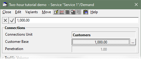
Figure 3: The Connections section of the
Demand dialog for the service
Note: it is not necessary to click in the formula bar to enter a value, or to click
the tick box to complete it. Just select the input you wish to edit and start typing,
and then press <Enter> when you are finished, or press <Tab> to move
on to the next input.
The Customer Base is straightforward to enter as
a constant value, whereas we want to enter the Penetration
input as a time series so that it will evolve over time as indicated:
-
Right click the Penetration input.
A context menu is displayed.
-
Select Change Type. A cascading sub-menu
appears, listing time-series alternatives such as Constant,
Straight Line, and so on.
-
Select S-Curve. An
S-Curve dialog is displayed.
-
Enter the essential six inputs as shown below (disregarding the Options).
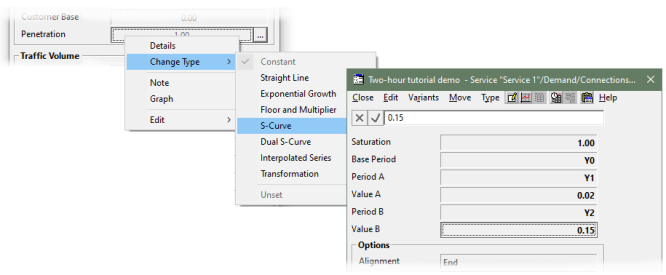
Figure 4: Entering S-Curve parameters for the Penetration input
The parameters are interpreted as follows:
- Saturation = 1.0 indicates
that we aim to connect every potential subscriber eventually (i.e., 100%)
- Base Period = Y0 directs
that the curve should start from zero in Y0
- Value A = 0.02 specifies
the level in Period A = Y1,
and similarly
- Value B = 0.15 the level
in Period B = Y2
- (each of these values to pertain at the end of the period by default).
We can easily preview the inferred curve and corresponding numbers:
- Click the Graph button
 on the dialog menu (or, if you prefer, select Graph
from the Move menu, or press <Alt+G>). A
graph of the Penetration input is displayed.
on the dialog menu (or, if you prefer, select Graph
from the Move menu, or press <Alt+G>). A
graph of the Penetration input is displayed.
-
Right-click the background of the graph and select
Show Separate Table (or select the same command from the graph
Format menu). A corresponding table is displayed.
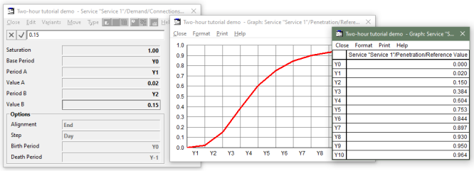
Figure 5: Drawing a graph and the associated table of the
Penetration input
The graph provides the best overview of the time-series evolution, while the table
allows you to check the inferred values in individual years. Are they as you expected?
 Things that you should have seen and understood
STEM Model Editor (‘the Editor’), toolbar, service
element, Demand
Connections Unit, Customer Base, Penetration
Change Type, S-Curve
Graph, Table