Watch the video presentation and/or read the full text below
Now we are going to run the model and draw the first results graphs.
Note: if you haven’t saved the model yet, you will be prompted to do so now.
-
Select [Save and] Run from the
File menu (or press <F5>). The model is first
checked for consistency and viability. STEM detects a potential problem, and prompts
with a Yes/No
choice, Model has input data warnings. Continue?
-
Click No to see what happens. A message
is displayed in the Editor, warning that our
Service has no Requirements.
Don’t worry; we will soon address this!
For now, we just want to review the impact of the service assumptions entered so
far.
-
Run the model again, and this time, at the warning prompt, click Yes to continue. The model is run and the Results
program loads, initially with a blank canvas, within which we will graph some results.
-
Select Draw… from the Graphs menu. The Draw
dialog is displayed, with tabs for Elements, Graphs and Format.
The first tab lists the Available elements as (Network) and our service Broadband
connectivity.
-
Select Broadband connectivity in
the list, and then click the Graphs tab. The service
is automatically added to the Selected list, and
then the Graphs tab is displayed, listing the available
Graphs to draw.
-
Select Connections in the list and
then press OK. A graph is drawn, showing the evolution
of the result over the ten-year run period. This should have the same shape as the
graph of the Penetration input that we drew earlier,
but scaled up by the 1000 of the Customer Base
input. Are the actual numbers what you expect?
-
Right-click the background of the graph and select
Show Separate Table (or select the same command from the main
Format menu). A corresponding table is displayed. You should see
that there are 20 customers in Y2 (2%) and 150 customers in Y3 (15%). (These may
differ if you still have shorter time-period inputs from earlier on.)
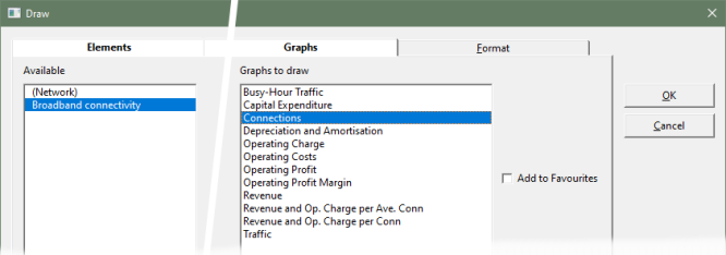
Figure 11: Selecting from the Elements and
Graphs tabs in the Draw dialog
This trivial graph illustrates the difference between the input domain of the Editor
and the calculated output domain of the Results program.
We will check the traffic outputs next, and learn two essential shortcuts at the
same time:
-
Select Draw Another… from the main
Graphs menu. The Draw
dialog is displayed, with the same element and graph selections as the
last graph drawn.
-
Go straight to the Graphs tab, this time
select Busy Hour Traffic, and press
OK. The graph is drawn. With a contention
ratio of 10, the nominal 100 Mbit/s service will average to 10 Mbit/s per
customer in aggregate across the 1000 customers, so the peak traffic should
approach 10 Gbits/s. Does your graph reflect this?
-
Select Draw Similar… from the main
Graphs menu (or right-click the background of either
graph to access the same command). The Draw dialog
is displayed, with the same element and graph selections as the
current graph.
-
Go straight to the Graphs tab again, and
now draw Traffic (i.e., volume). The graph is drawn.
That’s a lot of data! The limit should be something like 10 × 60 ×
60 / 8 / 1024 / 0.2 × 250 ~ 10 × 0.44 / 0.2 × 250 = 4.4 ×
1250 = 5500 Tbytes (i.e., 5.5 Pbytes).
-
Select Tile from the
Graphs menu to tidy the presentation. The three graphs are tiled in the
order of most recently active. Try experimenting with this.
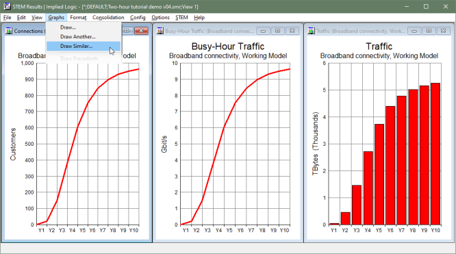
Figure 12: Connections and traffic results for the
Broadband connectivity service
 Things that you should have seen and understood
Run, warnings, Results program
Draw, Elements, Graphs
Draw Another, Draw Similar
Connections, Busy Hour Traffic, Traffic