Exercise 44: Working Capital

Close the Results program and whichever model you currently have open in the Editor, and then re-open WiMAX-DSL02.

Before we change anything, we are going to have a closer look at the timing of the monies flowing in or out of the business.

1. Select Draw New… from the Graphs menu. The Edit Graph Definition dialog is displayed.
2. Choose Network for the type of result, and then select Cashflow before Financing from the list of results.

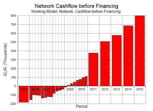
Note: the default setting is to show Y0 in line charts only. You should select the Show Y0 option from the main Consolidation menu to show Y0 for this particular chart.

Why is this non-zero in year zero (2005)? Let’s find out!

Draw precedents

3. Press <F2> to draw precedents for this graph, and repeat this process to step back through Cashflow from Operations, Pre-Tax Profit, Operating Profit, Operating Costs, and then Rental Cost.

All of these results are network results, but the network Rental Cost result is an aggregation over all resources. So when you draw precedents for Rental Cost, you will be prompted to choose one or more resources.

4. Since you don’t know where the cost is coming from, click Set All in the Choose elements to draw dialog, and also select All elements on one graph. A graph showing Rental Cost for all resources is drawn, which should answer the question above.

What can you do to fix this? Hint: think about which services require backhaul bandwidth. For which of these is the demand independent of the number of subscribers? Simply change one of the service user data so that the demand does not commence until Y1.

In the next group of exercises (on cost allocation) you will learn how to query directly which services are using a given network asset.

5. Close the various precedents graphs until you get back to Precedents of Cashflow from Operations.

Here you should note that the Pre-Tax Profit in Q1 2006 is somewhat offset by Change in Debtors less Creditors. This is because, by default, STEM assumes an average of thirty days for payment terms on all operating costs. In the early days of the business, this acts as a slight cushion and means that the Cashflow before Financing is less negative in Q1 2006 than it would be otherwise.

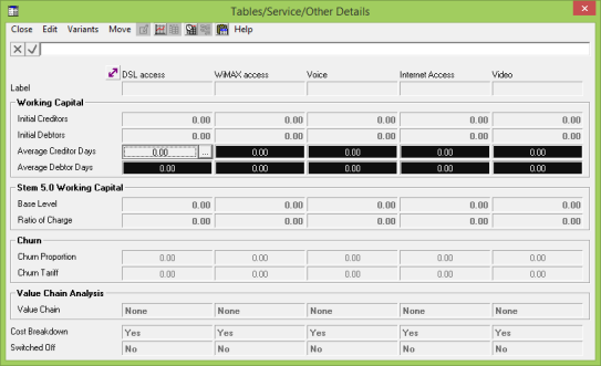
This assumption is controlled at the service level. In the Other Details dialog you will see inputs for both Average Creditor Days and Average Debtor Days.

6. Go to the Other Details dialog (icon menu/Advanced/Other Details) for one of the services, and then click the button on the dialog menu to view a tabular dialog with one column for each of the five services.
7. Set Average Creditor Days = 0.0 for one of the services and then use copy and paste to copy this value onto both Average Creditor Days and Average Debtor Days for all services.

8. Re-run the model and note the impact on Cashflow from Operations.

Later in the development of the business, when services are profitable and revenues are increasing, the impact of Average Debtor Days can be seen.

9. Note the exact value of Cashflow from Operations in 2015 with the Average Debtor Days set to zero as above.
10. Return the Average Creditor Days and Average Debtor Days inputs for all services to their default values (dialog Edit menu/Unset, or press <Del> with each cell selected), and re-run the model.

How has Cashflow from Operations changed?

A business must have sufficient fluidity in its finances, known as ‘working capital’, to provide for the net difference between the timing of receipts and payments.

Please disregard the STEM 5.0 Working Capital inputs, which are only there for backwards compatibility.