Exercise 47: Financial instruments (Debt Facilities)

By default, STEM models long-term borrowing with an infinitely flexible ‘float’ which attracts interest according to the Borrowing Rate input. This float is increased on demand to provide as much borrowing as is required by the target gearing constraint, and is paid off progressively and without penalty as soon as the business generates sufficient surplus cash.

In reality, a venture may have approved financing from one source up to a negotiated ceiling, and for any additional funding may then have to turn to alternative and more expensive sources. Such a debt facility may typically have a non-trivial fee structure, and a pre-determined repayment schedule. We will now show how this can be modelled in STEM.

Debt facility

1. Click the button on the toolbar and click again within the view to create a new debt facility. Name it Vendor finance.
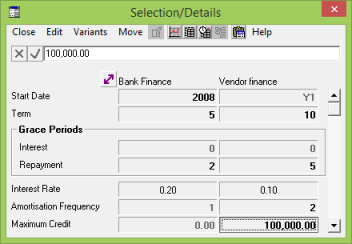
2. Set the inputs Term = 10, Repayment = 5 and Interest Rate = 0.1 (icon menu/Details).

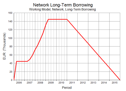
3. Look at the Network Long-Term Borrowing graph again. You should see that the debt balance now increases monotonically to its limit (around EUR145 000) and then decreases only gradually from Y6 to Y10.

Amortisation frequency

4. Change the input Years in Quarters to 10 and re-run the model (Data menu/Run Period).

You will see that the balance is actually paid off in five annual tranches.

5. Change the input Amortisation Frequency = 2 and re-run the model (debt facility icon menu/Details).

Now the repayments are made every six months, i.e., twice a year.

Maximum credit

6. Set the input Maximum Credit = 100,000.0 and re-run the model (debt facility icon menu/Details).

You will see the balance temporarily exceed the EUR100 000 ceiling.

7. Draw the graph Debt Facility Balance, and also a new graph for the network result, Long-Term Borrowing Float.

The fallback, flexible float mentioned above kicks in for the excess debt.

8. Create another debt facility and name it Bank finance.
9. Populate its inputs as shown below and re-run the model.

10. Draw the graph Debt Facility Balance, with both debt facilities on the same graph.

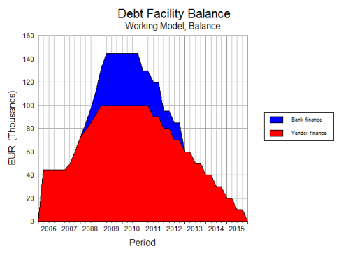
You will see that Bank finance is now used for the extra funding, and this is paid back over three years.

How does STEM split the additional funding from the beginning of 2008? (Compare the balances between Q4 2007 and Q1 2008.)

Mapping

You can use the Mapping input for each debt facility to define what share of the incremental borrowing each should satisfy, which is useful to model parallel loans from multiple sources, or a pre-defined calendar switch. However, this cannot be used to switch over automatically when one source of credit is exhausted.

Sequence

11. Set the input Sequence Index = 1 for the Bank finance element and re-run the model (debt facility icon menu/Details).

Now STEM only considers Bank finance (and any other debt facility with the same sequence index) when the credit from Vendor finance is exhausted.

12. Reduce the term for Bank finance to 3 years, set the Amortisation Frequency to 4 and re-run the model.

Now the Bank finance is repaid over one year.

13. Draw the graphs Debt Facility Balance and Debt Facility Interest Expense, with both debt facilities on the same graph, and tile the two graphs side-by-side as shown below.

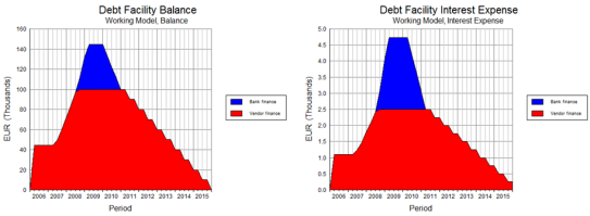
You can see the disproportionate impact of the more expensive financing from the bank. In a real-life simulation, this would allow you to model the consequences of an over-ambitious roll-out plan or customer-acquisition strategy.

14. If there is time, experiment with the interest grace period and various fees for each of the debt facility elements.