Exercise 3: Modify an input and run the model

To complete our high-level understanding of working with STEM, we are going to change one of the inputs and see how it affects the results.

1. Select Editor from the STEM menu in the Results program, or click the Editor tab in the Windows taskbar, or press <Alt+Tab> to switch back to the Editor.

Global data

For simplicity, we are going to change one of the global assumptions in the model, namely the 60% of homes within reach of the available DSL technology, together with the granularity of the run period of the model.

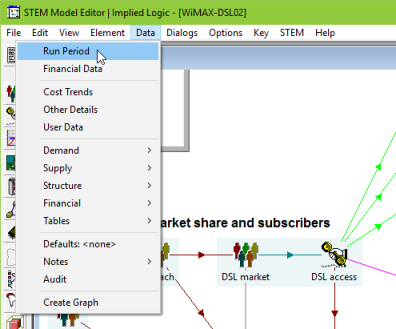
The element-specific data are accessed from the associated icon menus, whereas the global inputs are accessed from the main menu:

2. Select Data from the main menu in the Editor. The Data menu is displayed.

3. Select Run Period. The Run Period dialog is displayed.

Run Period

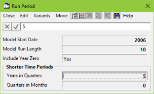
These inputs govern the time domain for the model – ten years from 2006, with 2005 as year zero – and the granularity of results generated.

4. Use the cursor-down (down arrow) key, or click in the cell as shown, to select the Years in Quarters field.
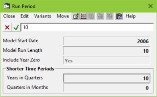
5. Enter ‘10’. The focus will switch to the formula bar and the buttons will be enabled.

6. Press <Enter> or click to accept the change.

It is not necessary to click in the formula bar to start editing; the focus shifts automatically when you start typing. Press <F2> if you want to modify (rather than replace) the existing text.

7. Close the Run Period dialog.
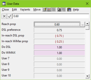
8. Select User Data from the Data menu. The global User Data dialog is displayed.

User Data

User Data are provided as an extension to the core STEM model inputs and enable you to fully customise a model with your own specific parameters which can be linked in turn through to the core inputs via formulae. (We shall explore this process thoroughly in a later exercise.)

The first field has been named as Reach prop (short for proportion). The value 0.6 indicates that 60% of homes are within reach of the available DSL technology.

Almost all STEM inputs can be time series, and we shall change this number to increase over time as the technology is improved. Notice that for a chosen cell/input field in this dialog, a small button appears on the right; we shall see how to quickly enter constant values, and more generally, how to enter time series.

9. Use the cursor keys or click to select the Reach prop cell.
10. Type the higher value of 0.8 and press <Enter>. The cell changes to read 0.80.
11. Click on the small button to the right of the main Reach prop field to enter the Constant dialog for the Reach prop field (or press <Enter> while the main field is selected).

Time series inputs

12. Select Type from the dialog menu. A range of parameterisations is offered, from each of which a time-series can be generated. We will experiment with these different types throughout the exercises.

Interpolated Series

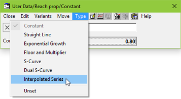
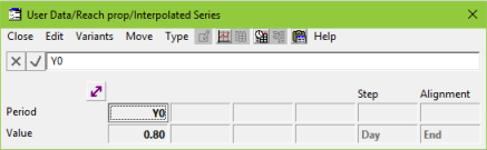
13. For now, select Interpolated Series (as the next easiest choice to understand and work with after Constant). An Interpolated Series dialog is displayed.

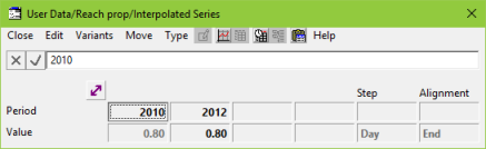
14. Change Y0 to 2012, and then enter 2010 in the next empty Period. (Don’t forget to press <Enter> to commit the 2012 change first.)

You can press <Tab> to commit an edit and move directly to the next cell in an any data dialog.

When you commit the 2010 change, the columns are automatically sorted in chronological order, putting the 2010 first. You will see that the same value of 0.8 is shown in grey for 2010.

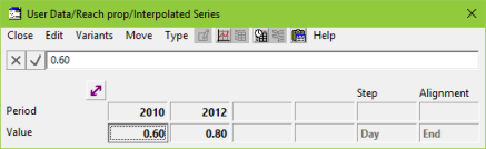
15. Change the value of 0.8 to 0.6 for 2010 and press <Enter>.

Graphing a time-series input

16. Click the button on the dialog menu, or press <Alt+G>. A graph is displayed showing how the parameters are interpreted.

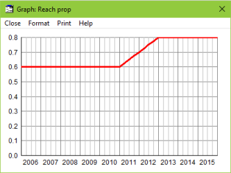
As the name suggests, STEM performs a linear interpolation between the given inputs, and makes a constant extrapolation up to the first period and on from the last period.

Press <F1> on the Interpolated Series dialog (or any time-series dialog) to get more background on how these time-series inputs work.

17. As we want to use our predefined graphs for DSL, which rely on the scenario DSL/Base, we need to run the corresponding scenario. For simplicity, use <Shift + F5> to access the Scenarios and Sensitivities dialog and run the selection.

View 1 appears, which is empty, so switch to the DSL architecture view (View menu/DSL architecture), where we would expect to see the effect of the increased DSL reach. It is clear that more DSL ports are required, a further DSL shelf is required and the utilisation of the DSLAM chassis increases from 80% to 100% (all five shelves filled).

18. Switch back to the Editor.
19. Close the graph window.
20. Close the Interpolated Series dialog for the Reach proportion. Spend some time getting used to navigation within the User Data dialog.

Right-clicking on a field brings up a drop-down menu allowing you to Change Type (e.g., to an Interpolated Series) and opens the corresponding input dialog. Pressing <Enter> in a selected field or clicking the small button to the right of the field also opens the associated time-series dialog, where you can change values or Type of time-series directly.