STEM offers two alternative ways of calculating the unit Capital Cost of a Resource in years other than the Calibration Period. A global flag determines whether the Cobb-Douglas production function is used (the default) or the Zero-Elasticity production function, which is easier to understand.
Zero-Elasticity production function
In the simpler case, the proportions of each Cost Index remain fixed in time and the unit cost is calculated as a weighted sum of the various Cost Indices included in the Cost Structure:
The unit cost in year n, Cn, is given by:
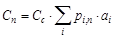
where
Cc
= calibration cost of the Resource
pi,n = value of Cost Index
i in year
n
ai
= proportion of Cost Index i.
In this case, the Capital Cost Structure proportions, ai, remain constant with time. The breakdown of the Resource by physical component does not change, as substitution between these components is not allowed.
Cobb-Douglas production function
The alternative function fixes the relative proportions of the production cost due to each Cost Index, no matter how the various trends vary.
Here the unit cost is given by:
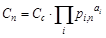 (1)
(1)
where again
Cc
= calibration cost of the Resource
pi,n = value of Cost Index
i in year
n
ai
= proportion of Cost Index i, which can be thought of as the elasticity of cost component
i
to a change in its price.
This approach is based on minimising the cost function, Cn(x), in each year n:
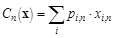
where
xi,n
= the quantity of cost component i in the Resource in year n,
subject to the constraint of constant production, Qn, in year n:
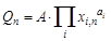
where
A = a calibration constant.
The quantities, xi,n, are given by the following equation:
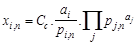
which can be re-arranged, substituting from (1), to confirm that the proportion of cost contributed by Cost Index
i
remains constant:

In this case, substitution between the physical components occurs as the relative quantities of components that are getting cheaper are increased against the relative quantities of those which are getting more expensive. The Cobb-Douglas production function assumes that any cost component can be substituted for another included in the Resource’s Cost Structure, while the proportions,
ai, of the Resource unit cost due to each Cost Index remain constant, despite differing cost trends for the various Cost Indices.
Example
We now examine a numerical application. Consider a Resource with two cost components, hardware and software, with hardware accounting for
60%
of the original unit cost and software for 40%. Let us assume that the unit cost of the Resource in the first year is
100. In the second year, we assume that the hardware price is divided by two while the software price is divided by four.
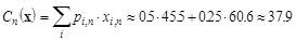
Using the Zero-Elasticity model, the physical proportions of hardware and software remain
0.6
and 0.4 respectively and the Resource cost in the second year is:
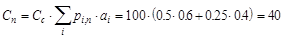
whereas with the Cobb-Douglas model, the quantities in the second year are:
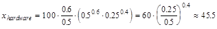
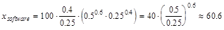
and the cost of the Resource decreases to:
As expected, the proportion of hardware decreased and the proportion of software increased: hardware is replaced by software as the price of software drops at a faster rate. As a result of the optimisation, the unit cost of the Resource is lower than in the Zero-Elasticity model above.
As a second illustration, consider a Resource with two Cost Indices; one accounts for
90%
of the unit cost in the Calibration Period and has a constant price trend; the other accounts for
10%
and becomes 50% cheaper every year. If the Calibration Period is
Year 5
and the unit cost of the Resource in that year is 100, the costs given by the two production functions are as shown in the Figure below.
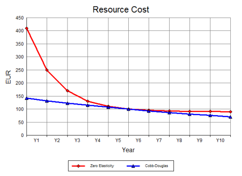
Unit Capital Cost with different production functions
With the Zero-Elasticity production function, a change in any one of the Cost Indices included in the Cost Structure may cause a large change in the unit cost of the Resource. With the Cobb-Douglas production function, the effect is limited, as the resource proportions are adjusted to minimise the unit cost. (The case chosen for this illustration is more extreme than you would normally find.) However, the unit capital cost is always lower in the Cobb-Douglas model than in the Zero-Elasticity model, because cost components are optimised every year in the latter so as to give the lowest unit cost possible.