By default, the Penetration and Traffic per Connection inputs define the actual demand used in the model. However, both these quantities can be related separately to each of the Connection, Rental and Usage Tariffs, so that the actual demand is scaled from the inputs, according to the actual tariffs charged.
Reference tariff
The feedback mechanism is based on the principle that the demand inputs are assumptions which must be qualified by corresponding assumptions about tariffs. These assumptions are known as reference demand and reference tariffs respectively, ideally based on market research on the Penetration, or Traffic per Connection, to be expected at a given set of tariffs.
The actual demand is calculated by scaling the reference demand, according to proportional changes in the actual tariffs charged
–
which may be either cost dependent or cost independent –
compared to the respective reference tariffs.
Price elasticity
Defines the proportional change in demand which will arise from a proportional change in tariff. A zero value signifies that demand is not influenced by tariff at all, while an elasticity of 1.0 means that a 1% decrease in tariff would generate approximately a 1% increase in demand.
The particular value of 1 causes demand to change in inverse proportion to tariff, which means that revenue is then unaffected by such changes. The actual values used should be based on observed characteristics of the market you are modelling.
The actual demand, AD, is calculated as follows:
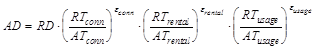
where
ATi = actual tariff i
RD = reference demand
RTi = reference tariff i
εi
= Price Elasticity with respect to tariff i
i
= Connection, Rental or Usage.
The same form of this equation is used for both Penetration and Traffic per Connection, but you can specify the Reference Tariffs and Elasticities for each measure of demand separately. The elasticities may well be different in real life, and the reference Penetration and Traffic per Connection may be based on different tariff assumptions.
The equation above which relates tariff and demand makes some assumptions about the nature of the market, and the shape of the price/quantity demand curve used by economists. It is assumed that elasticity is constant in any one year, but changing over time, so that you are, in effect, defining a series of curves describing the movement of price against quantity, as shown below.
Demand ratio
Each of the terms, (RT/AT)ε, used to scale the reference demand in the equation above, are generated as Demand Ratio results in their own right, e.g., Penetration/Rental Demand Ratio, providing a useful indication of how Tariff Feedback to Demand is working in your model. Clearly the further the actual demand varies from the reference demand, the more speculative the results are likely to be; and so it is worth checking that individual Demand Ratios stay reasonably close to 1.
Tariff/demand curves
In a simple illustration, we assume that customer behaviour, e.g., disposable income, does not change with time. From a market research study, we know that a given reference tariff would produce a given reference demand. The elasticity is constant at 1, so any change from the reference tariff generates a corresponding change from the reference demand. The actual tariff is assumed to be a cost dependent tariff, decreasing by a constant amount every year. The corresponding increase in demand is illustrated on the single tariff/demand curve below.
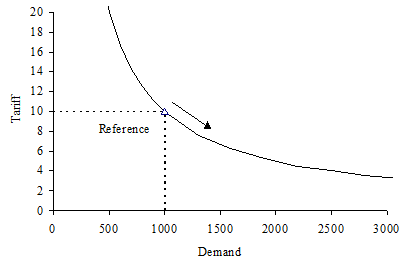
Figure 1: Constant Reference assumptions and falling Actual Tariff
In a more general case, we assume that customer behaviour changes with time. This is modelled by variable decreasing reference tariffs and reference demands (specifying time series for the Service Reference Tariff and Penetration or Traffic per Connection inputs). The elasticity coefficient is assumed to be constant.
In the following graph, each tariff/demand curve represents customer behaviour for one year, and the curve is moving to the right as time progresses. The shape of the curve reflects the elasticity coefficient, and is a measure of how customers would react to variations in tariff in a given year. The triangles mark the reference demand and reference tariff assumptions in each year. The bullets indicate the actual tariffs charged and the associated demand.
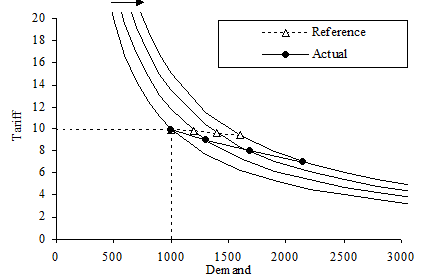
Figure 2: Varying Reference assumptions and falling Actual Tariff
When setting up a model, you should remember that the relationship between reference tariff, reference demand and elasticity describes a series of curves of this type, and that the shifts in these curves over time represent changes in customer behaviour. If you set a reference demand which is increasing at the same time as the reference tariff is increasing, you are assuming either that more people want your service, or that they have more money to spend on it.
Instability
It is possible to construct a model in which feedback will cause demand and tariff to oscillate. This may occur when elasticity is high, the charge per connection depends on demand, and the Initial Cost Dependent Tariff is very different from the tariff calculated from costs. To control the instability you must either correct the value for the initial tariff, or specify a tariff Maximum Change, to limit the actual changes in tariff
–
and hence demand – from one year to the next.
Effect of elasticity on demand and revenue
The graphs below illustrate the extent to which demand and revenue depend on tariff, according to different elasticities. Both graphs show normalised variables, i.e., tariff, demand and revenue (tariff
´
demand) divided by their reference values.
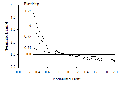
Figure 3: Effect of Elasticity on Demand
The Elasticity parameter defines the extent to which the actual charged tariff affects the demand (and, in turn, the revenue). Here are some specific examples:
-
Elasticity = 0.0 means there is no feedback at all and demand will not be affected by the charged tariff; revenue is increased directly if tariff is increased
-
Elasticity = 0.5: if the tariff is increased by a factor of x > 1, then the demand is reduced by the lesser x0.5 (i.e., √x) and the overall revenue is increased by a factor √x
-
Elasticity = 1.0: the demand is reduced by x1.0 (i.e., x), meaning that the demand varies in inverse proportion to the tariff (and by implication the overall revenue remains the same); e.g., if the charged tariff is twice the assumed reference tariff, then the demand is halved and the revenue product is the same
-
Elasticity = 2.0: the demand is reduced by the greater x2.0 (i.e., x2) and the overall revenue is decreased by the factor x.
| Elasticity |
Actual tariff charged as a proportion of reference tariff |
|
0.5 |
0.75 |
1.00 |
1.50 |
2.00 |
| 0.0 |
1.00 |
1.00 |
1.00 |
1.00 |
1.00 |
| 0.5 |
1.41 |
1.15 |
1.00 |
0.82 |
0.71 |
| 1.0 |
2.00 |
1.33 |
1.00 |
0.67 |
0.50 |
| 2.0 |
4.00 |
1.78 |
1.00 |
0.44 |
0.25 |
Figure 4: The demand ratio is dependent on the actual tariff charged and the elasticity parameter
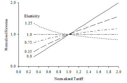
Figure 5: Effect of Elasticity on Revenue