STEM allows for various scenarios which will impact on the calculation of depreciation, making it possible to:
- assign a Residual Value
to an asset
- specify a Depreciation Schedule
as an explicit time series
- bring forward the depreciation schedule of an asset in a case where its business life is re-planned (Calendar Override).
Residual Value
When modelling the depreciation of an asset, its value is normally spread over a period of time, at the end of which the asset is considered to have zero value. There are cases, however, in which it may be possible to sell the asset when it is no longer needed in the network. For example, an operator might buy a GSM base station now, with the intention of selling this on to another country in 5 years when the operator is ready to upgrade its own technology. The price obtained is the
Residual Value
of the asset, captured in the Costs dialog.
In such cases, where you anticipate that you will be able to sell the asset, it would be unreasonable to depreciate more than the difference between the initial value of the asset and the sell-on price (the Residual Value), because the effective cost to the business is only the difference between these. An extreme example is that of land, which is typically not included as a business cost because its value generally appreciates rather than depreciates, making its residual value greater than its capital cost.
Depreciation is calculated based on an estimate of what the residual value will be when a resource is removed from the network. However, this may occur earlier than anticipated if the resource becomes redundant, in which case a correction may be required to the final depreciation.
There are two associated results:
- Proceeds from Sale of Assets
is the positive cash flow item that arises when the Resource is sold.
- Profit on Sale of Assets
arises if the Resource is sold for more than its net book value: it is equal to the cash received from the sale minus the written-down value of the Resource after its final depreciation. This will normally be zero, but could be positive if the Resource is removed early and is sold for a higher price than the original estimated residual value.
In addition, there are two predefined graphs, Network Sale of Assets and
Resource Sale of Assets, each of which includes these two results.
Depreciation Schedule
When specifying how depreciation should be spread over the financial lifetime of a Resource, STEM provides an alternative to the Straight Line or Reducing Balance options, namely to specify a Depreciation Schedule as an explicit time series in the Financial Details dialog. This feature allows you to match any non-standard or statutory depreciation methods, such as the Modified Accelerated Cost Recovery System (MACRS) used in the USA.
For example, the following input would defer depreciation for 2 years, until the Resource was actually operational. A constant of
1.0
(the default) is equivalent to Straight Line depreciation.
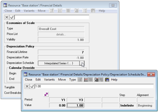
Setting up a Depreciation Schedule as a time series
The depreciation schedule as entered is subsequently normalised at run-time, in order to integrate to 1.0 over the financial lifetime.
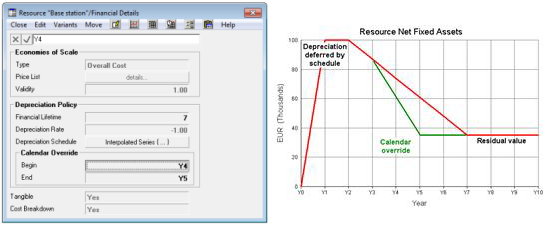
Calendar Override
Calendar Override is provided as a way to revise the timing of depreciation in a scenario where the business life of an asset is re-planned. For example, a resource installed in Y1 may have been depreciated initially with a Financial Lifetime of 7 years, but then the availability of a new technology may lead management to plan its early replacement. So in Y4 you may wish to bring forward the original depreciation schedule, anticipating an earlier removal by the end of Y5. This calendar override applies to all installed ages of equipment: so newer equipment in Y2 will be depreciated more quickly to satisfy the calendar override.