If you are modelling a new network, the core infrastructure of backbone network and switching must be installed before you can credibly model any connections to, or traffic on, this network. Suppose network roll-out is assumed to commence at the beginning of the year and you want to investigate the cashflow implications for when in the first year of operations you can start connecting customers. In order to demonstrate this with a small model with one Service requiring one Resource:
- Select Tariffs from the icon menu for the Service. The Tariffs dialog appears.
- Enter a nominal, constant value of 1.5 for the Rental Tariff.
- Select Demand from the dialog Move menu. The Demand dialog appears.
- Click the Penetration field, and enter S-Curve or Interpolated Series data such that demand grows from a zero value at the end of
Q2
– see Figure 3 below.
- Enter a constant value of, for example, 10,000 in the Customer Base field.
- Now select Capacity and Lifetime from the icon menu for the Resource. The Capacity and Lifetime dialog is displayed.
- Enter a value of 5 for the Physical Lifetime.
- Select Costs from the dialog Move menu. The Costs dialog appears.
- Enter a nominal value of 1.0 for the Capital Cost.
- Select Advanced/Other Details from the dialog Move menu. The Other Details dialog is displayed, with a Planned Units field that represents a minimum total installation constraint for the end of each period of the model run.
- Select the Planned Units field and enter an Interpolated Series with zero at the end of
Y0
and target values for Y1 and beyond – see Figure 3 below.
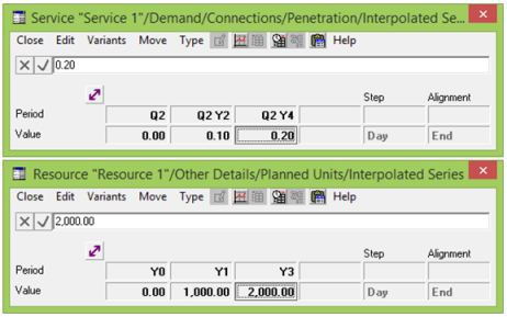
Figure 1: Using Planned Units as Advance Installation Data
- Select Save and Run from the File menu. The model is saved and calculations commence. When the run is complete, the results are loaded into the Results program.
- Select Draw from the Graphs menu in the Results program. The Draw Graphs dialog is displayed.
- Select Resource Installed Units, Service Demand in Connections and Network Revenue and Expenditure, and then click OK. The graphs are drawn.
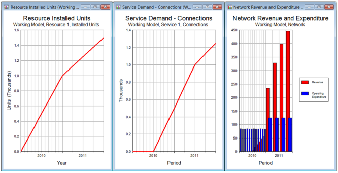
Figure 2: Cashflow implications of Advance Installation
As you can see, equipment is installed gradually from the beginning of Y1, ahead of the actual Service demand, which doesn’t start until Q3. This means that there is no revenue for the first six months.
Now you can define scenarios for the Service penetration, perhaps varying the introduction of service between Q2, Q3 and Q4 – see 9.3 Working with scenarios. If you run all of these scenarios, you can then draw Network Cash Balance in order to compare the cumulative cashflow effects of these three scenarios.
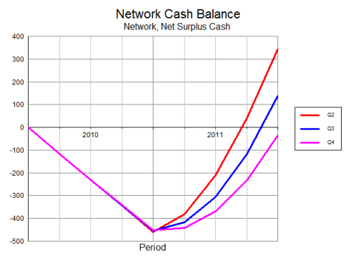
Figure 3: Cashflow implications of delayed introduction of Service
Note: The Planned Units input represents a minimum constraint on the total installation of a Resource during the model run. This is in marked contrast with the pre-run Installation Profile input, which prescribes incremental units for each of the pre-run years – see 10.3.21 Pre-Run Installation.