In order to illustrate the key features of the shorter time period model, we will construct a simple model comprising one Service:
-
target market of 100 potential customers
-
Penetration rising quickly from 0% in 2000 to 40% in 2002; and then, more slowly, to 50% in 2005,
requiring one Resource:
-
Capacity of 16.0 connections
-
Physical Lifetime of 3 years.
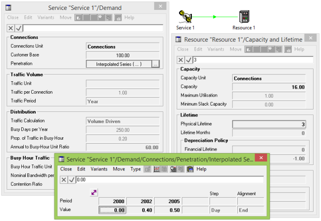
Figure 1: Simple model
Adding detail to the Run Period
First define the time frame for the model with a Model Start Date of 2001 and Model Run Length of 5 years. Year zero is included by default, so if you draw a graph of Service Penetration by clicking on the
 button in the Interpolated Series dialog, you will see that the model runs from years 2000 to 2005 inclusive.
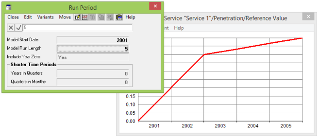
Figure 2: Annual Run Period
Now superimpose further detail on the run period by setting the optional inputs Years in Quarters =
1
and Quarters in Months = 1. Additional data are plotted for Jan, Feb and Mar, Q2, Q3 and Q4 of 2001, reflecting the actual periods for which results will be calculated when the model is run.
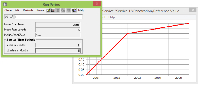
Figure 3: Run Period with Months and Quarters
Note: The shorter time period data are plotted closer together, reflecting the relative lengths of the corresponding periods. This behaviour is enabled via a Proportional Spacing checkbox in the Format Graph dialog. Otherwise the data are plotted evenly spaced, which is useful if you want to zoom in on the initial data.
Running the model
STEM can perform calculations for an arbitrary series of periods, although the current interface limits this to a number of initial months and quarters, with an optional base year.
The model engine installs equipment at the beginning of a period to meet end-of-period demand. The most significant complication is that traffic, revenue and operating cost calculations must all take account of the length of each period (measured in days). For example, the Rental Revenue result for a given period is calculated as the product of the Rental Tariff input, average connections over the period, and the length of the period in years (i.e., the number of days divided by 360).
Examining some results
We will draw graphs of some familiar results:
-
Service Demand in Connections, which you will note is proportional to the Penetration input
-
Resource Installed and Incremental Units, which requires further analysis.
It is always good practice to verify the magnitude and timing of results to make sure you haven’t mistyped an input – a misplaced decimal can have a big impact! Here we can see that, by the end of 2005, four units have been installed, providing capacity of 4 × 16 = 64 connections which matches the corresponding demand of 50 connections, with 14 connections slack capacity.
If you draw a table of the Service Demand, you can then see that the number of connections first goes past 16 in Q4 2001, hence the second installed unit, and past 32 in 2002, hence the third, but not past 48 until 2005.
You can almost check the number of incremental units against the change in installed units, except for the complication of replacement. The two units installed in Jan 2001 and Q4 2001 are both replaced in 2004, and the single unit installed in 2002 is replaced in 2005.
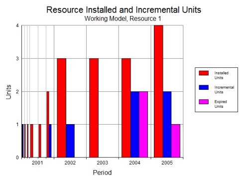
Figure 4: Resource Installed and Incremental Units
As you can see, the introduction of shorter time periods to the model calculations immediately leads to more detail in the results, without having to alter, re-structure or complicate the input data.
Consolidation
The ‘raw’ results shown above reflect the shorter time periods used by the model engine, and are essential for analysing the model results. However, just as important is the requirement to compare and report consolidated annual results – see 5.5 Consolidating monthly or quarterly results.
- Select one of the graphs you have drawn.
Click on the Consolidation menu in the Results program. A choice of Year, Quarter or Month is presented.
-
Select Year. The selected graph is re-drawn, with the results for Jan, Feb and Mar, Q2, Q3 and Q4 of 2001 all replaced by a single value.
Note: selecting the All Graphs menu item on the Consolidation menu takes you to a Consolidation dialog where you may chose additionally for the selected consolidation mode to Apply To the current or all views (see 5.5 Consolidating monthly or quarterly results).
If you compare the impact on installed and incremental units, you will see that installed units take the end-of-period (Q4 2001) value, whereas incremental units are summed over the period (Jan through Q4 2001). This reflects the fact that the installed units result represents the total number installed at the end of a period, whilst the incremental units value represents the number actually installed during a period.
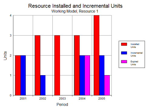
Figure 5: Consolidation in Years
If you select Quarter from the Consolidation menu, as much quarterly detail is presented as possible. So, in this case, Jan, Feb and Mar 2001 are consolidated to Q1 2001, followed by the raw Q2, Q3 and Q4 2001. However, the subsequent results are still shown annually, as the requisite quarterly data is not available.
Note: It would be very misleading for the system to make any attempt to estimate quarterly results, e.g., by interpolation or dividing the raw annual results by four. If you require additional quarterly results, simply increase the Years in Quarters input for the run period.