It is important for any investment model to establish clear definitions of the results it calculates, particularly regarding the timing of demand and the installation of equipment. Just like its annual predecessor, the STEM 6.0 model engine installs equipment at the beginning of a period to match end-of-period demand.
The additional requirement to mix monthly, quarterly and annual data, both in the input data and in the actual model calculations, makes this precision paramount. The elapsed time between successive periods, say Mar and Q2, depends crucially on whether you are measuring from the beginning or the end of those periods. This concept of alignment within a period goes right to the heart of the evaluation of parameterised time-series inputs and the subsequent model calculations.
Elapsed days from the model start date
The Model Start Date is entered as a period, which can be either a year (implying
1 Jan), or a fully qualified date if you want to model in financial years, e.g., from
5 Apr 2001. The actual date is implicitly aligned to the beginning of the specified period; and to be precise, in the two cases given, the first year of the model runs from midnight at the beginning of 1 Jan Y1 (or 5 Apr 2001) to midnight at the
end of 30 Dec Y1 (or 4 Apr 2002).
Whenever the value of any other input is specified for a period, an alignment must be given, either implicitly or explicitly, in order to resolve precisely when the input should assume the given value in terms of elapsed days into the model run.
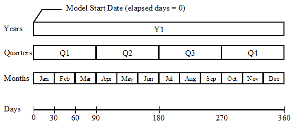
Figure 1: Elapsed days to the Beginning or End of a Period
For example, in a calendar model: the beginning of Q2 (midnight at the beginning of 1 Apr) is 90 days into the model run, whilst the end of Q2 (midnight at the end of 30 Jun) represents 180 elapsed days.
Calibration Period for Services and Resources
Service and Resource elements both have Calibration Period inputs that are used to fix administrative costs and costs in time. Related cost trends are then used to calculate values in other periods. Because the model engine installs equipment at the
beginning
of a period to match demand at the end of a period, it evaluates cost trends at the beginning of a given period. Consequently, the Calibration Period inputs have an
implicit
beginning-of-period alignment. This means that if, e.g., you define Calibration Period =
Y1
for a Resource, you will find that the various costs take their calibration values at the beginning of Y1, i.e., Q1 or Jan, and higher values in Q2 to Q4 if you have defined increasing cost trends.
Default alignment for demand, tariffs and cost trends
All the other period inputs are parameters for the various time-series types, such as Exponential Growth, Floor and Multiplier, S-Curve and Interpolated Series. Each of these parameterisations has an explicit Alignment input that allows you to qualify whether the calibration data are beginning-of-period or end-of-period.
Again, because the model engine installs equipment at the beginning of a period to match end-of-period demand, time-series inputs for demand have
End alignment by default, whereas both tariff and cost trend data have
Beginning alignment by default. The significance of this Alignment for the various types is explained in the following sections, as well as the implications of using non-default Alignment.
Base Period for Exponential Growth and Floor and Multiplier inputs
In an annual model, a time-series input specified as an Exponential Growth takes its Base value in year zero by default, and grows each year by an amount governed by the Multiplier input. Now an explicit Base Period input can be used to specify a particular period when the input should assume the Base value.
Note: The base year for Exponential Growth and Floor and Multiplier inputs in STEM 5.4 was implicitly year zero; with the obscure exception of Service tariff data, for which the base year was the Service Calibration Period.
Suppose we take a time-series input with default End Alignment, such as Service Penetration, and define it as an Exponential Growth with input Base =
0.5
and input Multiplier = 1.05, representing 5% annual growth. If you plot a graph of the time series, you will see that it takes the value 0.5 in Y0 and grows thereafter.
If you now change the value of the Base Period input from the default
Y0
to Y1, you will see from the graph that the time-series takes a lower value in Y0, achieving the Base value of 0.5 in Y1.
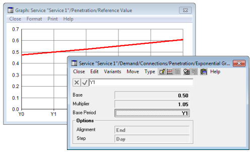
Figure 2: Base Period for Exponential Growth
End alignment
Now if you add shorter time periods to the model, e.g., by setting the run period input Years in Quarters = 1, you can see the significance of the
End
Alignment: the Base value is achieved in Q4, i.e., at the end of Y1 – see Figure 3 below. Lower values pertain for Q1 to Q3.
The way that STEM calculates these values is to measure the number of elapsed days between the end of a given period and the end of the specified Base Period. So the Base value is associated with midnight at the end of Y1, and values are calculated for midnight at the end of the respective quarters. This method produces a set of values which match the conventional annual interpretation whilst providing sensible intermediate values for the shorter time periods.
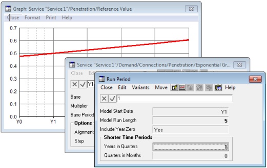
Figure 3: End-Aligned Exponential Growth
Beginning alignment
For a time-series input with default Beginning
Alignment, such as Service Rental Tariff, a similar logic would identify the beginning of Y1 with the beginning of Q1, so that the input would take the value 0.5 in Q1, with higher values in Q2 to Q4.
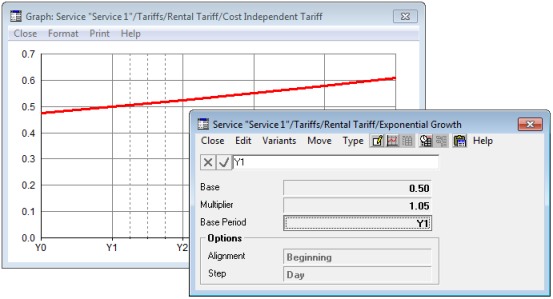
Figure 4: Beginning-Aligned Exponential Growth
Exactly the same general logic governs the interpretation of the Base Period for a time-series input specified as a Floor and Multiplier, and also, as explained below, the interpretation of the various calibration periods for S-Curves and Interpolated Series.
Aligning against default
However, suppose you set Alignment = Beginning
for the Penetration input. Whilst this will tie the Base value of 0.5 to the beginning of Y1, the graph will now show this value for the period Y0. This is because the graph always reflects the values used by the model engine, which in this case will calculate demand for the end of Y0, which of course coincides with the beginning of Y1.
It is important to keep in mind the fact that the model engine must
use a consistent set of assumptions in order to validate the calculations it makes. The initially unintuitive behaviour of a graph of this kind of input simply reflects the mapping the system must make where necessary from beginning to end-of period values, or vice versa. Because of the potential for confusion, it is not recommended to use non-default Alignment unless you have data that specifically require it.
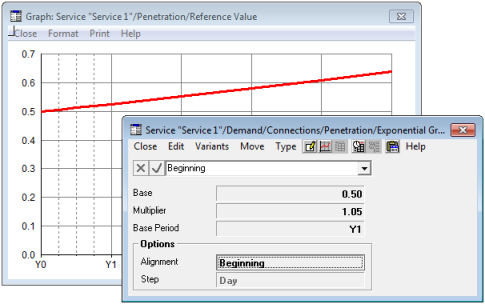
Figure 5: Aligning against Default
Periods for Interpolated Series
Each value in an Interpolated Series is now associated with a period, which may be a year or a quarter or whatever. Suppose you define Service Penetration to be
0.0
in Y0 and 1.0 in
Y10. This will clearly yield a value of 0.1 for Y1; and if you include quarters, the default
End
Alignment will tie this to Q4, i.e., the end of Y1, with proportionately lower values for Q1 to Q3.
The input values are tied to the end of Y0 and Y10 respectively, and for any intermediate period, a value will be interpolated according to the number of elapsed days between the end of Y0, the end of that period, and the end of Y10.
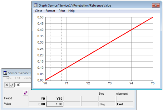
Figure 6: Using Elapsed days to interpolate Values
Periods for S-curve inputs
Three period inputs are used to fix the evolution of an S-Curve in time: the Base Period, Period A and Period B. If you define Service Penetration to be an S-Curve with Saturation =
1.0
and values 0.1 in Y1 and
0.5
in Y2, then again the default End
Alignment will tie the Y1 value of 0.1 to Q4, i.e., the end of Y1, with lower values in Q1 to Q3.
The input values are tied to the ends of Y1 and Y2 respectively, and indeed, the base point for the S-Curve is tied to the end of Y-1, which is the default Base Period. The S-Curve is fitted through these points and then a value for [the end of] any other period can be calculated to match that curve.
An S-Curve has two optional input parameters, the Birth Period and Death Period, which are used to ‘switch on’ or ‘switch off’ a time-series input in specified periods. Regardless of the explicit Alignment for the S-Curve, both these optional periods are always given a beginning-of-period interpretation, to match the intuitive expectation that, e.g., Service Penetration with Birth Period =
Y3
will take non-zero values throughout Y3 and thereafter, rather than from the end of Y3, and similarly that Death Period =
Y7
will force zero values for the whole of Y7 and beyond.
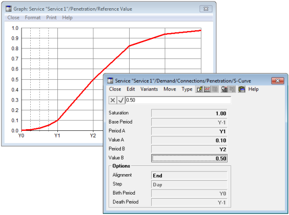
Figure 7: Using Elapsed days to calculate S-Curve Values
Linking time-series inputs with opposite alignment
One time-series input can be linked to another, either by entering a simple reference formula, or by using the Copy and Paste Link commands – see 4.14.4 Linking default values for inputs governed by several parameters. The input with the formula will inherit its Alignment and other parameters from the other input. So if this technique is used to link inputs with opposite Alignment, then one of the two inputs will be aligned against default, with the resulting behaviour described above.
For example, if you choose to enter MaxUtilisation
as a formula for the Maintenance Cost Trend for a Resource, in order to link default values from the Maximum Utilisation input, the cost trend will inherit parameters with End Alignment. Thus a calibration value for Maximum Utilisation, e.g., specified for [the end of] Y1, will be assumed by the cost trend at [the beginning of] Y2.
However, it is most unlikely that you would actually want to link demand inputs at face value to tariffs or cost trends, or vice versa, so this whole scenario is fortunately rather contrived and of little practical concern.
Evaluating numeric expression for time-series inputs
In addition to the alternative time-series parameterisations, you can define a time series with a numeric formula, using operators and functions to combine numbers and other time-series data. When a time series is determined by an arithmetic formula, the usual parameterisation is replaced by a read-only table of values for each period of the model run – see 4.7.3 Time-series formulae. The resulting values are interpreted by the model engine as if constant throughout each of the corresponding periods, so a given time-series formula will yield the same values regardless of the implicit Alignment of the input to which it is applied.
If the formula refers to another time-series input which is defined with one of the concise parameterisations above, then, in order to evaluate the formula for a given period of the model run, an appropriate value for that input must be first calculated from its parameters. The parameterised input’s default alignment is applied so as to match the value used by the model engine for that input in the same period. Thus, arithmetic formulae will always relate the values used by the model engine for various inputs as expected, regardless of the respective alignments.
For example, suppose you have a Service with Penetration defined as an Interpolated Series with values 0.0 in Y0 and 1.0 in Y10. You could add a competing Service, with Penetration defined as a numeric formula:
1 – "Service 1".Penetration.RefValue
In order to calculate the explicit value for this formula in, e.g., Y1, STEM would first calculate the penetration for Service 1 in Y1, i.e., the interpolated value for the
end
of Y1, and then subtract this value from one.
Alternatively, suppose you relate Service Penetration to Rental Tariff, an input with opposite alignment, via a numeric formula that gives a penetration of 50% with elasticity of 0.1 relative to a reference tariff of 20:
0.5 * (20 / Tariffs.Rental.CostIndepTariff) ^ 0.1
Suppose further that the Rental Tariff is specified as an Exponential Growth with Base = 20 in Y0 and Multiplier = 0.95, representing a 5% annual drop. In order to calculate the penetration in, e.g., Y1, STEM would first calculate the tariff in Y1, i.e., the exponential value for the
beginning
of Y1, 20 ×
0.95 = 19, and then feed this into the expression above.