This transformation allows you to define a non-linear relationship between elements of a model. The Transformation takes the defined Input, and applies a user-defined Mapping to calculate its Output, which can then govern the installation of other equipment.
The Mapping that transforms the Input is defined very much like a time-series input, except that the Mapping is a function of the Input rather than time. The most useful Mapping is an Interpolated Series, which consists of a series of Input–Output pairs. Output values are interpolated linearly for Input values between these points, and extrapolated as a constant outside the range of Inputs given. For example, the Interpolated Series shown below could be used to limit demand to 1000, equivalent to an Output mapping:

where x
= Transformation Input, assumed to be non-negative.
| Input |
0.0 |
1000.0 |
| Output |
0.0 |
1000.0 |
Figure 1: Input–Output Mapping to limit Demand to 1000
As an example of using an Input–Output Mapping transformation in a real model, consider the problem of installing links to create a meshed network between a number of nodes. Assume that we have a Transformation,
Nodes, whose Output is the number of nodes. We create another Transformation,
Links, with Nodes as its Input and the Input–Output Mapping specified as follows:
| Input |
1.0 |
2.0 |
3.0 |
4.0 |
5.0 |
6.0 |
| Output |
0.0 |
1.0 |
3.0 |
6.0 |
10.0 |
12.0 |
Figure 2: Input–Output Mapping for a meshed network
This mapping creates a fully meshed network for up to five nodes. The sixth node is remote and would be connected to only two other nodes.
The Input values should extend as far as the maximum number of nodes that will exist in the model. The
Links
Transformation can now be mapped onto a Link
Function to provide the necessary number of links between the nodes.
As a more complex example of an Input–Output Mapping, suppose a switch requires cards mounted in cabinets. Each cabinet can contain up to 25 cards but must contain a minimum of five cards. Each card can support 20 units of demand. Thus the equipment required for various levels of demand is as shown below:
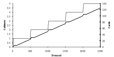
Figure 3: Cabinets and cards required for Demand
We first dimension the cabinets and cards, giving them capacities of 500 (20
×
25) and 20 respectively. We can then define a Location representing the minimum numbers of cards required, and use it to govern the Deployment of the cards.
The size of the Location is determined by an Input–Output Mapping Transformation, whose Input is the number of cabinets and whose Output is defined by the Mapping:
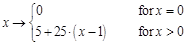
where
x
= Transformation Input, assumed to be non-negative.
(This rule is valid only if x
is an integer, but as the number of cabinets will always be an integer, this is not a problem.) Since this function is ‘almost linear’, it is easily defined by an Interpolated Series:
|
Input
|
0.0
|
1.0
|
20.0
|
| Output
|
0.0
|
5.0
|
480.0
|
Figure 4: Input–Output Mapping for minimum cards required
(The last Input value must be at least as large as the largest number of cabinets that will be installed in the model.)